
6.7.2: Using SAS
- Page ID
- 33830

\( \newcommand{\vecs}[1]{\overset { \scriptstyle \rightharpoonup} {\mathbf{#1}} } \)
\( \newcommand{\vecd}[1]{\overset{-\!-\!\rightharpoonup}{\vphantom{a}\smash {#1}}} \)
\( \newcommand{\dsum}{\displaystyle\sum\limits} \)
\( \newcommand{\dint}{\displaystyle\int\limits} \)
\( \newcommand{\dlim}{\displaystyle\lim\limits} \)
\( \newcommand{\id}{\mathrm{id}}\) \( \newcommand{\Span}{\mathrm{span}}\)
( \newcommand{\kernel}{\mathrm{null}\,}\) \( \newcommand{\range}{\mathrm{range}\,}\)
\( \newcommand{\RealPart}{\mathrm{Re}}\) \( \newcommand{\ImaginaryPart}{\mathrm{Im}}\)
\( \newcommand{\Argument}{\mathrm{Arg}}\) \( \newcommand{\norm}[1]{\| #1 \|}\)
\( \newcommand{\inner}[2]{\langle #1, #2 \rangle}\)
\( \newcommand{\Span}{\mathrm{span}}\)
\( \newcommand{\id}{\mathrm{id}}\)
\( \newcommand{\Span}{\mathrm{span}}\)
\( \newcommand{\kernel}{\mathrm{null}\,}\)
\( \newcommand{\range}{\mathrm{range}\,}\)
\( \newcommand{\RealPart}{\mathrm{Re}}\)
\( \newcommand{\ImaginaryPart}{\mathrm{Im}}\)
\( \newcommand{\Argument}{\mathrm{Arg}}\)
\( \newcommand{\norm}[1]{\| #1 \|}\)
\( \newcommand{\inner}[2]{\langle #1, #2 \rangle}\)
\( \newcommand{\Span}{\mathrm{span}}\) \( \newcommand{\AA}{\unicode[.8,0]{x212B}}\)
\( \newcommand{\vectorA}[1]{\vec{#1}} % arrow\)
\( \newcommand{\vectorAt}[1]{\vec{\text{#1}}} % arrow\)
\( \newcommand{\vectorB}[1]{\overset { \scriptstyle \rightharpoonup} {\mathbf{#1}} } \)
\( \newcommand{\vectorC}[1]{\textbf{#1}} \)
\( \newcommand{\vectorD}[1]{\overrightarrow{#1}} \)
\( \newcommand{\vectorDt}[1]{\overrightarrow{\text{#1}}} \)
\( \newcommand{\vectE}[1]{\overset{-\!-\!\rightharpoonup}{\vphantom{a}\smash{\mathbf {#1}}}} \)
\( \newcommand{\vecs}[1]{\overset { \scriptstyle \rightharpoonup} {\mathbf{#1}} } \)
\(\newcommand{\longvect}{\overrightarrow}\)
\( \newcommand{\vecd}[1]{\overset{-\!-\!\rightharpoonup}{\vphantom{a}\smash {#1}}} \)
\(\newcommand{\avec}{\mathbf a}\) \(\newcommand{\bvec}{\mathbf b}\) \(\newcommand{\cvec}{\mathbf c}\) \(\newcommand{\dvec}{\mathbf d}\) \(\newcommand{\dtil}{\widetilde{\mathbf d}}\) \(\newcommand{\evec}{\mathbf e}\) \(\newcommand{\fvec}{\mathbf f}\) \(\newcommand{\nvec}{\mathbf n}\) \(\newcommand{\pvec}{\mathbf p}\) \(\newcommand{\qvec}{\mathbf q}\) \(\newcommand{\svec}{\mathbf s}\) \(\newcommand{\tvec}{\mathbf t}\) \(\newcommand{\uvec}{\mathbf u}\) \(\newcommand{\vvec}{\mathbf v}\) \(\newcommand{\wvec}{\mathbf w}\) \(\newcommand{\xvec}{\mathbf x}\) \(\newcommand{\yvec}{\mathbf y}\) \(\newcommand{\zvec}{\mathbf z}\) \(\newcommand{\rvec}{\mathbf r}\) \(\newcommand{\mvec}{\mathbf m}\) \(\newcommand{\zerovec}{\mathbf 0}\) \(\newcommand{\onevec}{\mathbf 1}\) \(\newcommand{\real}{\mathbb R}\) \(\newcommand{\twovec}[2]{\left[\begin{array}{r}#1 \\ #2 \end{array}\right]}\) \(\newcommand{\ctwovec}[2]{\left[\begin{array}{c}#1 \\ #2 \end{array}\right]}\) \(\newcommand{\threevec}[3]{\left[\begin{array}{r}#1 \\ #2 \\ #3 \end{array}\right]}\) \(\newcommand{\cthreevec}[3]{\left[\begin{array}{c}#1 \\ #2 \\ #3 \end{array}\right]}\) \(\newcommand{\fourvec}[4]{\left[\begin{array}{r}#1 \\ #2 \\ #3 \\ #4 \end{array}\right]}\) \(\newcommand{\cfourvec}[4]{\left[\begin{array}{c}#1 \\ #2 \\ #3 \\ #4 \end{array}\right]}\) \(\newcommand{\fivevec}[5]{\left[\begin{array}{r}#1 \\ #2 \\ #3 \\ #4 \\ #5 \\ \end{array}\right]}\) \(\newcommand{\cfivevec}[5]{\left[\begin{array}{c}#1 \\ #2 \\ #3 \\ #4 \\ #5 \\ \end{array}\right]}\) \(\newcommand{\mattwo}[4]{\left[\begin{array}{rr}#1 \amp #2 \\ #3 \amp #4 \\ \end{array}\right]}\) \(\newcommand{\laspan}[1]{\text{Span}\{#1\}}\) \(\newcommand{\bcal}{\cal B}\) \(\newcommand{\ccal}{\cal C}\) \(\newcommand{\scal}{\cal S}\) \(\newcommand{\wcal}{\cal W}\) \(\newcommand{\ecal}{\cal E}\) \(\newcommand{\coords}[2]{\left\{#1\right\}_{#2}}\) \(\newcommand{\gray}[1]{\color{gray}{#1}}\) \(\newcommand{\lgray}[1]{\color{lightgray}{#1}}\) \(\newcommand{\rank}{\operatorname{rank}}\) \(\newcommand{\row}{\text{Row}}\) \(\newcommand{\col}{\text{Col}}\) \(\renewcommand{\row}{\text{Row}}\) \(\newcommand{\nul}{\text{Nul}}\) \(\newcommand{\var}{\text{Var}}\) \(\newcommand{\corr}{\text{corr}}\) \(\newcommand{\len}[1]{\left|#1\right|}\) \(\newcommand{\bbar}{\overline{\bvec}}\) \(\newcommand{\bhat}{\widehat{\bvec}}\) \(\newcommand{\bperp}{\bvec^\perp}\) \(\newcommand{\xhat}{\widehat{\xvec}}\) \(\newcommand{\vhat}{\widehat{\vvec}}\) \(\newcommand{\uhat}{\widehat{\uvec}}\) \(\newcommand{\what}{\widehat{\wvec}}\) \(\newcommand{\Sighat}{\widehat{\Sigma}}\) \(\newcommand{\lt}{<}\) \(\newcommand{\gt}{>}\) \(\newcommand{\amp}{&}\) \(\definecolor{fillinmathshade}{gray}{0.9}\)In SAS we would set up the ANOVA as:
proc mixed data=school covtest method=type3;
    class Region SchoolType Teacher Class;
    model sr_score = Region SchoolType Region*SchoolType;
    random Teacher(Region*SchoolType);
    store out_school;
run;
In SAS proc mixed, we see that the fixed effects appear in the model statement, and the nested random effect appears in the random statement.
We get the following partial output:
| Type 3 Analysis of Variance | ||||||||
|---|---|---|---|---|---|---|---|---|
| Source | DF | Sum of Squares | Mean Square | Expected Mean Square | Error Term | Error DF | F Value | Pr > F |
| Region | 1 | 564.062500 | 564.062500 | Var(Residual) + 2 Var(Teach(Region*School)) + Q(Region,Region*SchoolType) | MS(Teach(Region*School)) | 4 | 24.07 | 0.0080 |
| SchoolType | 1 | 76.562500 | 76.562500 | Var(Residual) + 2 Var(Teach(Region*School)) + Q(SchoolType,Region*SchoolType) | MS(Teach(Region*School)) | 4 | 3.27 | 0.1450 |
| Region*SchoolType | 1 | 264.062500 | 264.062500 | Var(Residual) + 2 Var(Teach(Region*School)) + Q(Region*SchoolType) | MS(Teach(Region*School)) | 4 | 11.27 | 0.0284 |
| Teach(Region*School) | 4 | 93.750000 | 23.437500 | Var(Residual) + 2 Var(Teach(Region*School)) | MS(Residual) | 8 | 5.00 | 0.0257 |
| Residual | 8 | 37.500000 | 4.687500 | Var(Residual) | . | . | . | . |
The results for hypothesis tests for the fixed effects appear as:
| Type 3 Tests of Fixed Effects | ||||
|---|---|---|---|---|
| Effect | Num DF | Den DF | F Value | Pr > F |
| Region | 1 | 4 | 24.07 | 0.0080 |
| SchoolType | 1 | 4 | 3.27 | 0.1450 |
| Region*SchoolType | 1 | 4 | 11.27 | 0.0284 |
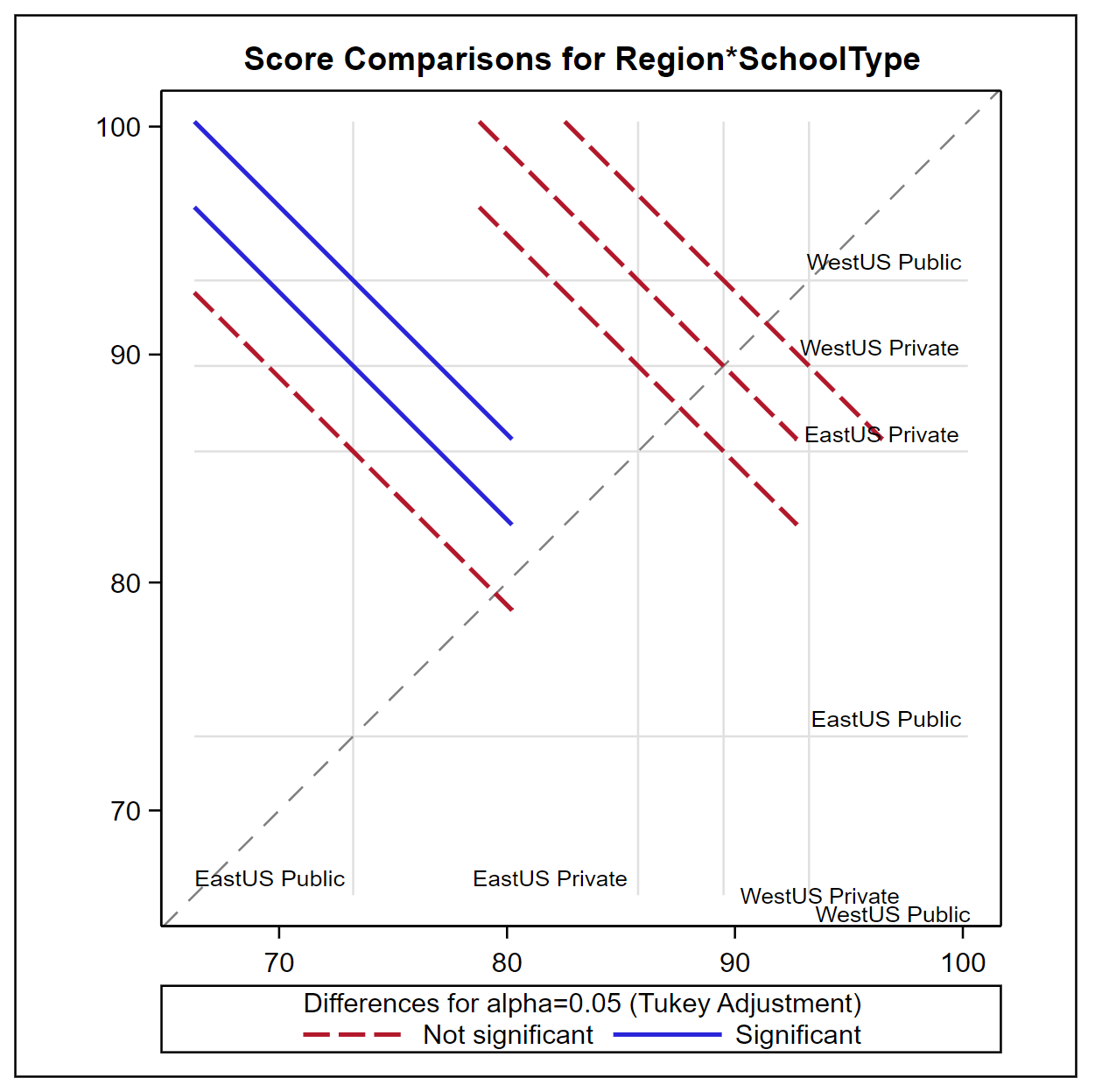
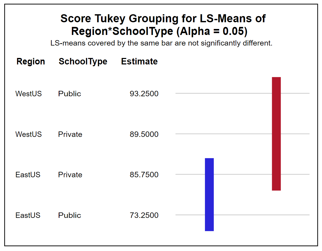
Given that the Region*SchoolType interaction is significant, the PLM procedure along with the lsmeans statement can be used to generate the Tukey mean comparisons and produce the groupings chart and the plots to identify what means differ significantly.
ods graphics on;
proc plm restore=out_school;
lsmeans Region*SchoolType / adjust=tukey plot=meanplot cl lines;
run;

| Differences of Region*SchoolType Least Squares Means Adjustment for Multiple Comparisons: Tukey |
||||||||||||||
|---|---|---|---|---|---|---|---|---|---|---|---|---|---|---|
| Region | SchoolType | _Region | _SchoolType | Estimate | Standard Error | DF | t Value | Pr > |t| | Adj P | Alpha | Lower | Upper | Adj Lower | Adj Upper |
| EastUS | Private | EastUS | Public | 12.5000 | 3.4233 | 4 | 3.65 | 0.0217 | 0.0703 | 0.05 | 2.9955 | 22.0045 | -1.4356 | 26.4356 |
| EastUS | Private | WestUS | Private | -3.7500 | 3.4233 | 4 | -1.10 | 0.3349 | 0.7109 | 0.05 | -13.2545 | 5.7545 | -17.6856 | 10.1856 |
| EastUS | Private | WestUS | Public | -7.5000 | 3.4233 | 4 | -2.19 | 0.0936 | 0.2677 | 0.05 | -17.0045 | 2.0045 | -21.4356 | 6.4356 |
| EastUS | Public | WestUS | Private | -16.2500 | 3.4233 | 4 | -4.75 | 0.0090 | 0.0301 | 0.05 | -25.7545 | -6.7455 | -30.1856 | -2.3144 |
| EastUS | Public | WestUS | Public | -20.0000 | 3.4233 | 4 | -5.84 | 0.0043 | 0.0146 | 0.05 | -29.5045 | -10.4955 | -33.9356 | -6.0644 |
| WestUS | Private | WestUS | Public | -3.7500 | 3.4233 | 4 | -1.10 | 0.3349 | 0.7109 | 0.05 | -13.2545 | 5.7545 | -17.6856 | 10.1856 |
.png?revision=1&size=bestfit&width=536&height=534)
.png?revision=1&size=bestfit&width=545&height=424)
From the results, it is clear that the mean self-rating scores are highest for the public school in the west region. The difference mean scores for public schools in the west region is significantly different from the mean scores for public schools in the east region as well as the mean scores for private schools in the east region.
The covtest option produces the results needed to test the significance of the random effect, Teach(Region*SchoolType) in terms of the following null and alternative hypothesis: \[H_{0}: \ \sigma_{teacher}^{2} = 0 \text{ vs. } H_{a}: \ \sigma_{teacher}^{2} > 0 \nonumber\]
However, as the following display shows, covtest option uses the Wald Z test, which is based on the \(z\)-score of the sample statistic and hence is appropriate only for large samples—specifically, when the number of random effect levels is sufficiently large. Otherwise, this test may not be reliable.
| Covariance Parameter Estimates | ||||
|---|---|---|---|---|
| Cov Parm | Estimate | Standard Error |
Z Value | Pr Z |
| Teach(Region*School) | 9.3750 | 8.3689 | 1.12 | 0.2626 |
| Residual | 4.6875 | 2.3438 | 2.00 | 0.0228 |
Therefore, in this case, as the number of teachers employed is few, Wald's test may not be valid. It is more appropriate to use the ANOVA \(F\)-test for Teacher(Region*SchoolType). Note that the results from the ANOVA table suggest that the effects of the teacher within the region and school type are significant (Pr > F = 0.0257), whereas the results based on Wald's test suggest otherwise (since the \(p\)-value is 0.2626).