
6.1: Random Effects
- Page ID
- 33658

When a treatment (or factor) is a random effect, the model specifications together with relevant null and alternative hypotheses will have to be changed. Recall the cell means model defined in Chapter 4 for the fixed effect case, which has the model equation: \[Y_{ij} = \mu_{i} + \epsilon_{ij}\] where \(\mu_{i}\) are parameters for the treatment means.
For the single factor random effects model we have: \[Y_{ij} = \mu_{i} + \epsilon_{ij}\] where \(\mu_{i}\) and \(\epsilon_{ij}\) are independent random variables such that \(\mu_{i} \overset{iid}{\sim} \mathcal{N} \left(\mu, \sigma_{\mu}^{2}\right)\) and \(\epsilon_{ij} \overset{iid}{\sim} \mathcal{N} \left(0, \sigma_{\epsilon}^{2}\right)\). Here, \(i = 1, 2, \ldots, T\) and \(j = 1, 2, \ldots, n_{i}\), where \(n_{i} \equiv n\) if balanced.
Notice that the random effects ANOVA model is similar in appearance to the fixed effects ANOVA model. However, the treatment mean \(\mu_{i}\)'s are constant in the fixed-effect ANOVA model, whereas in the random-effects ANOVA model the treatment mean \(\mu_{i}\)'s are random variables.
Note that the expected mean response, in the random effects model stated above, is the same at every treatment level and equals \(\mu\).
\[E \left(Y_{ij}\right) = E \left(\mu_{i} + \epsilon_{ij}\right) = E \left(\mu_{i}\right) + E \left(\epsilon_{ij}\right) = \mu\]
The variance of the response variable (say \(\sigma_{Y}^{2}\)) in this case can be partitioned as: \[\sigma_{Y}^{2} = V \left(Y_{ij}\right) = V \left(\mu_{i} + \epsilon_{ij}\right) = V \left(\mu_{i}\right) + V \left(\epsilon_{ij}\right) = \sigma_{\mu}^{2} + \sigma_{\epsilon}^{2}\] as \(\mu_{i}\) and \(\epsilon_{ij}\) are independent random variables.
Similar to fixed effects ANOVA model, we can express the random effects ANOVA model using the factor effect representation, using \(\tau_{i} = \mu_{i} - \mu\). Therefore the factor effects representation of the random effects ANOVA model would be: \[Y_{ij} = \mu + \tau_{i} + \epsilon_{ij}\] where \(\mu\) is a constant overall mean, and \(\tau_{i}\) and \(\epsilon_{ij}\) are independent random variables such that \(\tau_{i} \overset{iid}{\sim} \mathcal{N} \left(0, \sigma_{\mu}^{2}\right)\) and \(\epsilon_{ij} \overset{iid}{\sim} \mathcal{N} \left(0, \sigma_{\epsilon}^{2}\right)\). Here, \(i = 1, 2, \ldots, T\) and \(j = 1, 2, \ldots, n_{i}\), where \(n_{i} \equiv n\) if balanced. Here, \(\tau_{i}\) is the effect of the randomly selected \(i^{th}\) level.
The terms \(\sigma_{\mu}^{2}\) and \(\sigma_{\epsilon}^{2}\) are referred to as variance components. In general, as will be seen later in more complex models, there will be a variance component associated with each effect involving at least one random factor.
Variance components play an important role in analyzing random effects data. They can be used to verify the significant contribution of each random effect to the variability of the response. For the single factor random-effects model stated above, the appropriate null and alternative hypothesis for this purpose is: \[H_{0}: \ \sigma_{\mu}^{2} = 0 \text{ vs. } H_{A}: \ \sigma_{\mu}^{2} > 0\]
Similar to the fixed effects model, an ANOVA analysis can then be carried out to determine if \(H_{0}\) can be rejected.
The MS and the df computations of the ANOVA table are the same for both the fixed and random-effects models. However, the computations of the F-statistics needed for hypothesis testing require some modification.
Specifically, the F statistics denominator will no longer always be the mean squared error (MSE or MSERROR) and will vary according to the effect of interest (listed in the Source column of the ANOVA table). For a random-effects model, the quantities known as Expected Means Squares (EMS), shown in the ANOVA table below, can be used to identify the appropriate F-statistic denominator for a given source in the ANOVA table. These EMS quantities will also be useful in estimating the variance components associated with a given random effect. Note that the EMS quantities are in fact the population counterparts of the mean sums of squares (MS) that we are already familiar with. In SAS the proc mixed, method=type3 option will generate the EMS column in the ANOVA table output.
| Source | df | SS | MS | F | P | EMS (Expected Means Squares) |
|---|---|---|---|---|---|---|
| Trt | \(\sigma_{\epsilon}^{2} + n \sigma_{\mu}^{2}\) | |||||
| Error | \(\sigma_{\epsilon}^{2}\) | |||||
| Total |
Variance components are NOT synonymous with mean sums of squares. Variance components are usually estimated by using the Method of Moments where algebraic equations, created by setting the mean sums of squares (MS) equal to the EMS for the relevant effects, are solved for the unknown variance components. For example, the variance component for the treatment in the single-factor random effects discussed above can be solved as:
\[s_{\text{among trts}}^{2} = \frac{MS_{trt} - MS_{error}}{n}\]
This is by using the two equations:
\(MS_{error} = \sigma_{\epsilon}^{2}\)
\(MS_{trt} = \sigma_{\epsilon}^{2} + n \sigma_{\mu}^{2}\)
More about variance components...
Often the variance component of a specific effect in the model is expressed as a percent of the total variation of the variation in the response variable.
Another common application of variance components is when researchers are interested in the relative size of the treatment effect compared to the within-treatment level variation. This leads to a quantity called the intraclass correlation coefficient (ICC), defined as: \[ICC = \frac{\sigma_{\text{among trts}}^{2}}{\sigma_{\text{\text{among trts}}^{2} + \sigma_{\text{within trts}}^{2}}\]
For single random factor studies, \(ICC = \frac{\sigma_{mu}^{2}}{\sigma_{mu}^{2} + \sigma_{\epsilon}^{2}}\). ICC can also be thought of as the correlation between the observations within the group (i.e. \(\text{corr} \left(Y_{ij}, Y_{ij'}\right)\), where \(j \neq j'\). Small values of ICC indicate a large spread of values at each level of the treatment, whereas large values of ICC indicate relatively little spread at each level of the treatment:
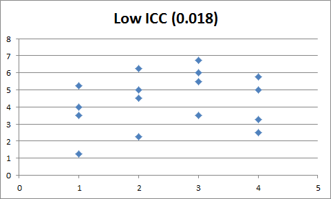.png?revision=1)
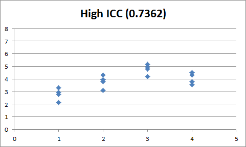.png?revision=1)