
2.6: Try It!
- Page ID
- 33186

To compare the teaching effectiveness of 3 teaching methods, the semester average based on 4 midterm exams from five randomly selected students enrolled in each teaching method were used.
- What is the response in this study?
- How many replicates are there?
- Write the appropriate null and alternative hypotheses.
- Complete the partially filled ANOVA table given below. Round your answers to 4 decimal places.
Source df SS MS F p-value teach_mtd 245 error total 345.1 - Find the critical value at \(\alpha = .01\)
- Make your conclusion.
- From the ANOVA analysis, you performed, can you detect the teaching method which yields the highest semester average? If not, suggest a technique that will.
- Solution
-
- Average of 4 mid-terms
- 5
- \(H_{0}: \ \mu_{1} = \mu_{2} = \mu_{3} = \mu_{4}\), where \(\mu_{1}, \mu_{2}, \mu_{3}\) are the actual semester average of a student enrolled in teaching method 1, method 2, and method 3 respectively. Ha: Not all semester averages are equal. (This means that there are at least two teaching methods that differ in their actual semester averages)
-
Source df SS MS F p-value teach_mtd 2 245 122.5000 14.6853 0.0006 error 12 100.1 8.3417 total 14 345.1 - 6.925
- As the calculated \(F\)-statistic value = 14.6853 is more than the critical value of 6.925, \(H_{0}\) should be rejected. Therefore, we can conclude that all 3 teaching methods do not have the same semester average, indicating that at least 2 teaching methods differ in their actual semester average.
- The ANOVA conclusion indicated that not all 3 teaching methods are equally effective, but did not indicate which one yields the highest mean score. The Tukey comparison method is one procedure that shows the teaching method that yields the significantly highest average semester score.
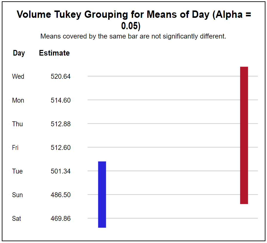
In a local commuter bus service, the number of daily passengers for 50 weeks was recorded. The purpose was to determine if the passenger volume is significantly less during weekends compared to workdays. Below are summary statistics for each day of the week. The partially filled ANOVA table, along with a Tukey plot, is shown below.
| Day | N | Mean | SE Mean | Std Dev |
|---|---|---|---|---|
| Sun | 50 | 486.500 | 9.003 | 63.661 |
| Mon | 50 | 514.600 | 6.891 | 48.724 |
| Tue | 50 | 501.340 | 7.922 | 56.018 |
| Wed | 50 | 520.640 | 7.055 | 49.886 |
| Thu | 50 | 512.880 | 10.258 | 72.532 |
| Fri | 50 | 512.600 | 8.086 | 57.174 |
| Sat | 50 | 469.860 | 8.988 | 63.555 |
a) State the appropriate null and alternative hypotheses for this test.
- Solution
-
\(H_{0}: \ \mu_{Sun} = \mu_{Mon} = \mu_{Tues} = \mu_{Wed} = \mu_{Thurs} = \mu_{Fri} = \mu_{Sat}\)
\(H_{A}: \ \text{At least one } \mu_{day \ i} \neq \mu_{day \ j}, \text{ for some\) i, j = 1, 2, \ldots, 7 \text{ OR not all means are equal}\)
b) Complete the partially filled ANOVA table given below. Use two decimal places in the \(F\) statistic.
| Source | df | SS | MS | F | p-value |
|---|---|---|---|---|---|
| Groups | 100391 | ||||
| Error | |||||
| Total | 1306887 |
- Solution
-
Source df SS MS F p-value Day 6 100391 16731.8 4.76 0.0001 Error 343 1206496 3517.5 Total 349 1306887
c) Use the appropriate \(F\)-distribution cumulative probabilities to verify that the \(p\)-value for the test is approximately zero.
- Solution
-
\(p\)-value \(\approx 0\) (from the \(F\)-distribution with 6 and 343 degrees of freedom)
d) Use \(\alpha=0.05\) to test if the mean passenger volume differs significantly by day of the week.
- Solution
-
Since the \(p\)-value \(\leq \alpha = 0.05\), we reject \(H_{0}\). There is strong evidence to indicate that the mean passenger volume differs significantly by day of the week (i.e., for some days of the week, the average number of commuters is more than others, but this test does not indicate which days have a higher passenger volume).
.png?revision=1&size=bestfit&width=566&height=515)
e) Use the output to make a statement about how the mean daily passenger volume differs significantly by day of the week.
- Solution
-
The passenger volume on Sundays is not statistically different from Saturdays and also from Tuesdays. The mean passenger volume on Saturdays is significantly lower than on workdays other than Tuesdays.
f) The management would like to know if the overall number of commuters is significantly more during workdays than during weekends. An appropriate comparison to respond to their query would be to compare the average number of commuters between workdays (Monday through Friday) and the weekend. Write the weight (coefficients) for a linear contrast to make this comparison. Test the hypothesis that the average commuter volume during the weekends is less.
- Solution
-
The weights (coefficients) for the appropriate contrast are given below.
Day Mon Tue Wed Thu Fri Sat Sun weight 1 1 1 1 1 -2.5 -2.5 \(t = \dfrac{\sum_{i=1}^{T} a_{i} \bar{y}_{i}}{\sqrt{MSE \sum_{i=1}^{T} \frac{a_{i}^{2}}{n_{i}}}} = \dfrac{171.16}{\sqrt{3517.5 * \frac{17.5}{50}}} = 4.878\)
Under the null hypothesis, this test statistic has a \(t\)-distribution with 343 degrees of freedom. You can obtain the \(p\)-value using statistical software. Recall this is a one-tailed test.
This \(p\)-value indicates that the difference in the average number of passengers is statistically significant between workdays and weekends.Student's t distribution with 343 DF \(x\) \(P(X \leq x)\) \(4.878\) \(8.216815 \cdot 10^{-7} \approx 0\) -
See the table below for computations:
Factor N Mean weights product weight2 Mon 50 514.6 1.0 514.6 1.00 Tue 50 501.34 1.0 501.34 1.00 Wed 50 520.64 1.0 520.64 1.00 Thu 50 512.88 1.0 512.88 1.00 Fri 50 512.6 1.0 512.6 1.00 Sat 50 469.86 -2.5 -1174.65 6.25 Sun 50 486.5 -2.5 -1216.25 6.25 Recall that the MSE (error mean squares) is 3517.5 with \(df_{error}=343\).