
2.4: Other Pairwise Mean Comparison Methods
- Page ID
- 33184

Although the Tukey procedure is the most widely used multiple comparison procedure, there are many other multiple comparison techniques.
An older approach, no longer offered in many statistical computing packages, is Fisher’s Protected Least Significant Difference (LSD). This is a method to compare all possible means, two at a time, as \(t\)-tests. Unlike an ordinary two-sample \(t\)-test, however, the method does rely on the experiment-wide error (the MSE). The LSD is calculated as: \[LSD(\alpha) = t_{\alpha, df} s_{\bar{d}}\] where \(t_{\alpha}\) is based on \(\alpha\) and \(df =\) error degrees of freedom from the ANOVA table. The standard error for the difference between two treatment means (\(s_{\bar{d}}\) or SE) is calculated as: \[s_{\bar{d}} = \sqrt{\frac{2s^{2}}{r}}\] where \(r\) is the number of observations per treatment mean (replications) and \(s^{2}\) is the MSE from the ANOVA. As in the Tukey method, any pair of means that differ by more than the LSD value differ significantly. The major drawback of this method is that it does not control \(\alpha\) over for an entire set of pair-wise comparisons (the experiment-wise error rate) and hence is associated with Type 1 inflation.
The following multiple comparison procedures are much more assertive in dealing with Type 1 inflation. In theory, while we can set \(\alpha\) for a single test, the fact that we have \(T\) treatment levels means there are \(T(T-1)/2\) tests (the number of pairs of possible comparisons), and so we need to adjust \(\alpha\) to have the desired confidence level for the set of tests. The Tukey, Bonferroni, and Scheffé methods control the experiment-wise error, but in different ways. All three use a \(\text{"multiplier"} * SE\) form, but differ in the form of the multiplier.
Contrasts are comparisons involving two or more factor level means (discussed more in the following section). Mean comparisons can be thought of as a subset of possible contrasts among the means. If only pairwise comparisons are made, the Tukey method will produce the narrowest confidence intervals and is the recommended method. The Bonferroni and Scheffé methods are used for general tests of possible contrasts. The Bonferroni method is better when the number of contrasts being tested is about the same as the number of factor levels. The Scheffé method covers all possible contrasts, and as a result, is the most conservative of all the methods. The drawback for such a highly conservative test, however, is that it becomes more difficult to resolve differences among means, even though the ANOVA would indicate that they exist.
When treatment levels include a control and mean comparisons are restricted to only comparing treatment levels against a control level, Dunnett’s mean comparison method is appropriate. Because there are fewer comparisons made in this case, the test provides more power compared to a test (see Section 3.7) using the full set of all pairwise comparisons.
To illustrate these methods, the following output was obtained (as we will see later on in the course) for the hypothetical greenhouse data of our example. We will be running these types of analyses later.
Fisher’s Least Significant Difference (LSD)
.png?revision=1&size=bestfit&width=729&height=636)
Since the estimated means for F1 and F3 are covered by the same colored bar, they are not significantly different using the LSD approach.
Tukey
.png?revision=1&size=bestfit&width=724&height=598)
Since the estimated means for F1 and F3 are covered by the same colored bar (red bar), they are not significantly different using Tukey's approach. Similarly, since F1 and F2 are covered by the same colored bar (blue bar) they are not significantly different using Tukey's approach.
Bonferroni
.png?revision=1&size=bestfit&width=724&height=594)
Observations from the Bonferroni approach are similar to the ones from Tukey's approach.
Scheffé
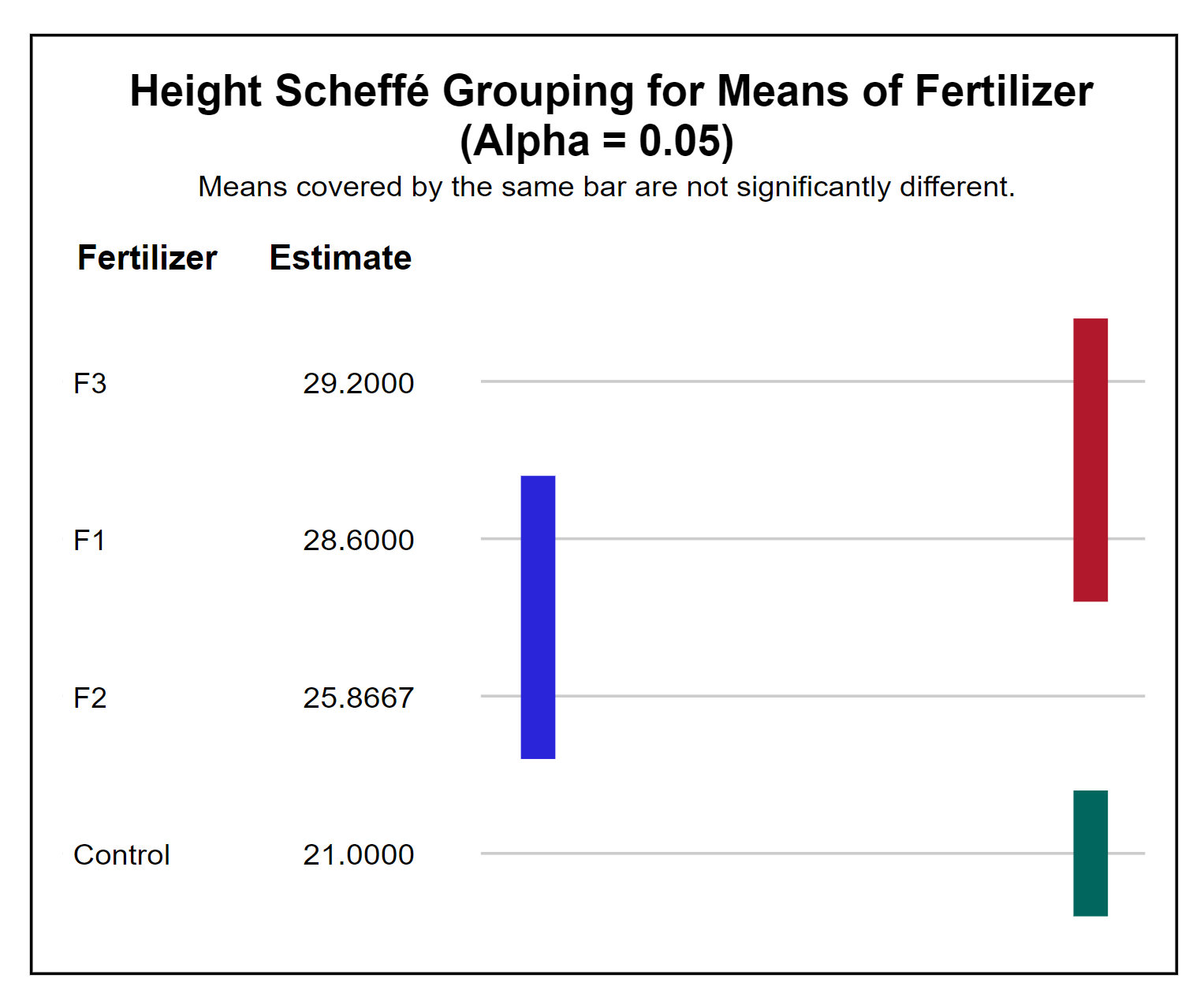.png?revision=1&size=bestfit&width=732&height=606)
Observations from the Scheffé approach are similar to the ones from Tukey's and Bonferroni's approaches.
Dunnett
| Comparisons significant at the 0.05 level are indicated by ***. | ||||
|---|---|---|---|---|
| Fertilizer Comparison |
Difference Between Means |
Simultaneous 95% Confidence Limits | *** | |
| F3 - Control | 8.200 | 5.638 | 10.762 | *** |
| F1 - Control | 7.600 | 5.038 | 10.162 | *** |
| F2 - Control | 4.867 | 2.305 | 7.429 | *** |
We can see that the LSD method was the most liberal, that is, it indicated the largest number of significant differences between means. In this example, Tukey, Bonferroni, and Scheffé produced the same results. The Dunnett test was consistent with the other 4 methods, and this is not surprising given the small value of the control mean compared to the other treatment levels.
To get a closer look at the results of employing the different methods, we can focus on the differences between the means for each possible pair:
| Comparison | Difference between means | |
|---|---|---|
| Control | F1 | 7.6000 |
| Control | F2 | 4.8667 |
| Control | F3 | 8.2000 |
| F1 | F2 | 2.7333 |
| F1 | F3 | 0.6000 |
| F2 | F3 | 3.3333 |
and compare the 95% confidence intervals produced:
| Type | LSD | Tukey | Bonferroni | Scheffé | Dunnett | ||||||
|---|---|---|---|---|---|---|---|---|---|---|---|
| Comparison | Lower | Upper | Lower | Upper | Lower | Upper | Lower | Upper | Lower | Upper | |
| Control | F1 | 5.496 | 9.704 | 4.777 | 10.423 | 4.648 | 10.552 | 4.525 | 10.675 | 5.038 | 10.162 |
| Control | F2 | 2.763 | 6.971 | 2.044 | 7.690 | 1.914 | 7.819 | 1.792 | 7.942 | 2.305 | 7.429 |
| Control | F3 | 6.096 | 10.304 | 5.377 | 11.023 | 5.248 | 11.152 | 5.125 | 11.275 | 5.638 | 10.762 |
| F1 | F2 | 0.629 | 4.837 | -0.090 | 5.556 | -0.2189 | 5.686 | -0.342 | 5.808 | X | X |
| F1 | F3 | -1.504 | 2.704 | -2.223 | 3.423 | -2.352 | 3.552 | -2.475 | 3.675 | X | X |
| F2 | F3 | 1.229 | 5.437 | 0.510 | 6.156 | 0.3811 | 6.286 | 0.258 | 6.408 | X | X |
You can see that the LSD produced the narrowest confidence intervals for the differences between means. Dunnett’s test had the next most narrow intervals, but only compares treatment levels to the control. The Tukey method produced intervals that were similar to those obtained for the LSD, and the Scheffé method produced the broadest confidence intervals.
What does this mean? When we need to be REALLY sure about our results, we should use conservative tests. If you are working in life-and-death situations, such as in most clinical trials or bridge building, you might want to be surer. If the consequences are less severe you can use a more liberal test, understanding there is more of a chance you might be incorrect (but still able to detect differences). In reality, you need to be consistent with the rigor used in your discipline. While we can't tell you which comparison to use, we can tell you the differences among the tests and the trade-offs for each one.