4.3: The Binomial Distribution
- Page ID
- 17326
\( \newcommand{\vecs}[1]{\overset { \scriptstyle \rightharpoonup} {\mathbf{#1}} } \)
\( \newcommand{\vecd}[1]{\overset{-\!-\!\rightharpoonup}{\vphantom{a}\smash {#1}}} \)
\( \newcommand{\id}{\mathrm{id}}\) \( \newcommand{\Span}{\mathrm{span}}\)
( \newcommand{\kernel}{\mathrm{null}\,}\) \( \newcommand{\range}{\mathrm{range}\,}\)
\( \newcommand{\RealPart}{\mathrm{Re}}\) \( \newcommand{\ImaginaryPart}{\mathrm{Im}}\)
\( \newcommand{\Argument}{\mathrm{Arg}}\) \( \newcommand{\norm}[1]{\| #1 \|}\)
\( \newcommand{\inner}[2]{\langle #1, #2 \rangle}\)
\( \newcommand{\Span}{\mathrm{span}}\)
\( \newcommand{\id}{\mathrm{id}}\)
\( \newcommand{\Span}{\mathrm{span}}\)
\( \newcommand{\kernel}{\mathrm{null}\,}\)
\( \newcommand{\range}{\mathrm{range}\,}\)
\( \newcommand{\RealPart}{\mathrm{Re}}\)
\( \newcommand{\ImaginaryPart}{\mathrm{Im}}\)
\( \newcommand{\Argument}{\mathrm{Arg}}\)
\( \newcommand{\norm}[1]{\| #1 \|}\)
\( \newcommand{\inner}[2]{\langle #1, #2 \rangle}\)
\( \newcommand{\Span}{\mathrm{span}}\) \( \newcommand{\AA}{\unicode[.8,0]{x212B}}\)
\( \newcommand{\vectorA}[1]{\vec{#1}} % arrow\)
\( \newcommand{\vectorAt}[1]{\vec{\text{#1}}} % arrow\)
\( \newcommand{\vectorB}[1]{\overset { \scriptstyle \rightharpoonup} {\mathbf{#1}} } \)
\( \newcommand{\vectorC}[1]{\textbf{#1}} \)
\( \newcommand{\vectorD}[1]{\overrightarrow{#1}} \)
\( \newcommand{\vectorDt}[1]{\overrightarrow{\text{#1}}} \)
\( \newcommand{\vectE}[1]{\overset{-\!-\!\rightharpoonup}{\vphantom{a}\smash{\mathbf {#1}}}} \)
\( \newcommand{\vecs}[1]{\overset { \scriptstyle \rightharpoonup} {\mathbf{#1}} } \)
\( \newcommand{\vecd}[1]{\overset{-\!-\!\rightharpoonup}{\vphantom{a}\smash {#1}}} \)
\(\newcommand{\avec}{\mathbf a}\) \(\newcommand{\bvec}{\mathbf b}\) \(\newcommand{\cvec}{\mathbf c}\) \(\newcommand{\dvec}{\mathbf d}\) \(\newcommand{\dtil}{\widetilde{\mathbf d}}\) \(\newcommand{\evec}{\mathbf e}\) \(\newcommand{\fvec}{\mathbf f}\) \(\newcommand{\nvec}{\mathbf n}\) \(\newcommand{\pvec}{\mathbf p}\) \(\newcommand{\qvec}{\mathbf q}\) \(\newcommand{\svec}{\mathbf s}\) \(\newcommand{\tvec}{\mathbf t}\) \(\newcommand{\uvec}{\mathbf u}\) \(\newcommand{\vvec}{\mathbf v}\) \(\newcommand{\wvec}{\mathbf w}\) \(\newcommand{\xvec}{\mathbf x}\) \(\newcommand{\yvec}{\mathbf y}\) \(\newcommand{\zvec}{\mathbf z}\) \(\newcommand{\rvec}{\mathbf r}\) \(\newcommand{\mvec}{\mathbf m}\) \(\newcommand{\zerovec}{\mathbf 0}\) \(\newcommand{\onevec}{\mathbf 1}\) \(\newcommand{\real}{\mathbb R}\) \(\newcommand{\twovec}[2]{\left[\begin{array}{r}#1 \\ #2 \end{array}\right]}\) \(\newcommand{\ctwovec}[2]{\left[\begin{array}{c}#1 \\ #2 \end{array}\right]}\) \(\newcommand{\threevec}[3]{\left[\begin{array}{r}#1 \\ #2 \\ #3 \end{array}\right]}\) \(\newcommand{\cthreevec}[3]{\left[\begin{array}{c}#1 \\ #2 \\ #3 \end{array}\right]}\) \(\newcommand{\fourvec}[4]{\left[\begin{array}{r}#1 \\ #2 \\ #3 \\ #4 \end{array}\right]}\) \(\newcommand{\cfourvec}[4]{\left[\begin{array}{c}#1 \\ #2 \\ #3 \\ #4 \end{array}\right]}\) \(\newcommand{\fivevec}[5]{\left[\begin{array}{r}#1 \\ #2 \\ #3 \\ #4 \\ #5 \\ \end{array}\right]}\) \(\newcommand{\cfivevec}[5]{\left[\begin{array}{c}#1 \\ #2 \\ #3 \\ #4 \\ #5 \\ \end{array}\right]}\) \(\newcommand{\mattwo}[4]{\left[\begin{array}{rr}#1 \amp #2 \\ #3 \amp #4 \\ \end{array}\right]}\) \(\newcommand{\laspan}[1]{\text{Span}\{#1\}}\) \(\newcommand{\bcal}{\cal B}\) \(\newcommand{\ccal}{\cal C}\) \(\newcommand{\scal}{\cal S}\) \(\newcommand{\wcal}{\cal W}\) \(\newcommand{\ecal}{\cal E}\) \(\newcommand{\coords}[2]{\left\{#1\right\}_{#2}}\) \(\newcommand{\gray}[1]{\color{gray}{#1}}\) \(\newcommand{\lgray}[1]{\color{lightgray}{#1}}\) \(\newcommand{\rank}{\operatorname{rank}}\) \(\newcommand{\row}{\text{Row}}\) \(\newcommand{\col}{\text{Col}}\) \(\renewcommand{\row}{\text{Row}}\) \(\newcommand{\nul}{\text{Nul}}\) \(\newcommand{\var}{\text{Var}}\) \(\newcommand{\corr}{\text{corr}}\) \(\newcommand{\len}[1]{\left|#1\right|}\) \(\newcommand{\bbar}{\overline{\bvec}}\) \(\newcommand{\bhat}{\widehat{\bvec}}\) \(\newcommand{\bperp}{\bvec^\perp}\) \(\newcommand{\xhat}{\widehat{\xvec}}\) \(\newcommand{\vhat}{\widehat{\vvec}}\) \(\newcommand{\uhat}{\widehat{\uvec}}\) \(\newcommand{\what}{\widehat{\wvec}}\) \(\newcommand{\Sighat}{\widehat{\Sigma}}\) \(\newcommand{\lt}{<}\) \(\newcommand{\gt}{>}\) \(\newcommand{\amp}{&}\) \(\definecolor{fillinmathshade}{gray}{0.9}\)The vast majority of the content in this book relies on one of five distributions: the binomial distribution, the normal distribution, the t distribution, the F distribution, and the χ2 (“chi-square”) distribution. Let's start with the binomial distribution, since it’s the simplest of the five. The normal distribution will be discussed later this chapter, and the others will be mentioned in other chapters. Our discussion of the binomial distribution will start with figuring out some probabilities of events happening.
Let’s imagine a simple “experiment”: in my hot little hand I’m holding 20 identical six-sided dice. On one face of each die there’s a picture of a skull; the other five faces are all blank. If I proceed to roll all 20 dice, what’s the probability that I’ll get exactly 4 skulls?
Let's unpack that last sentence. First, in case you missed it, rolling of the 20 dice is your sample. N = 20 (20 scores in this distribution). Second, it's asking about a probability, so we'll be looking back at the last section and realizing that we should do some division. Finally, this is a question, some might even call it a Research Question.
Okay, back to the "experiment." Assuming that the dice are fair, we know that the chance of any one die coming up skulls is 1 in 6; to say this another way, the skull probability for a single die is approximately .1667, or 16.67%.
\( {\dfrac1 6} = 0.166\overline {7} * 100 = 16.67% \)
The probability of rolling a skull with on die is 16.67%, but I'm doing this 20 times so that's
\( 0.166\overline {7} * 20 = 3.33 \) skulls
So, if I rolled 20 dice, I could expect about 3 of them to come up skulls. But that's not quite the Research Question is it? Let’s have a look at how this is related to a binomial distribution.
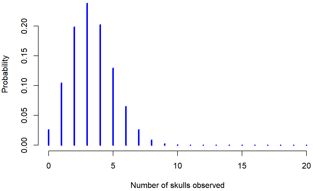
Figure \(\PageIndex{1}\) plots the binomial probabilities for all possible values for our dice rolling experiment, from X=0 (no skulls) all the way up to X=20 (all skulls). On the horizontal axis we have all the possible events (the number of skulls coming up when all 20 dice are rolled), and on the vertical axis we can read off the probability of each of those events. If you multiple these by 100, you'd get the probability in a percentage form. Each bar depicts the probability of one specific outcome (i.e., one possible value of X). Because this is a probability distribution, each of the probabilities must be a number between 0 and 1 (or 0% to 100%), and the heights of the all of the bars together must sum to 1 as well. Looking at Figure \(\PageIndex{1}\), the probability of rolling 4 skulls out of 20 times is about 0.20 (the actual answer is 0.2022036), or 20.22%. In other words, you’d expect to roll exactly 4 skulls about 20% of the times you repeated this experiment. This means that, if you rolled these 20 dice for 100 different repetitions, you'd get exactly 4 skulls in about 20 of your attempts.

Figure \(\PageIndex{1}\)- Probability of Rolling 4 Skulls out of 20 Dice with One Skull (CC-BY-SA Danielle Navarro from Learning Statistics with R)
Sample Size Matters
We'll be talking a lot about how sample size (N) affects distributions in this chapter, starting now!
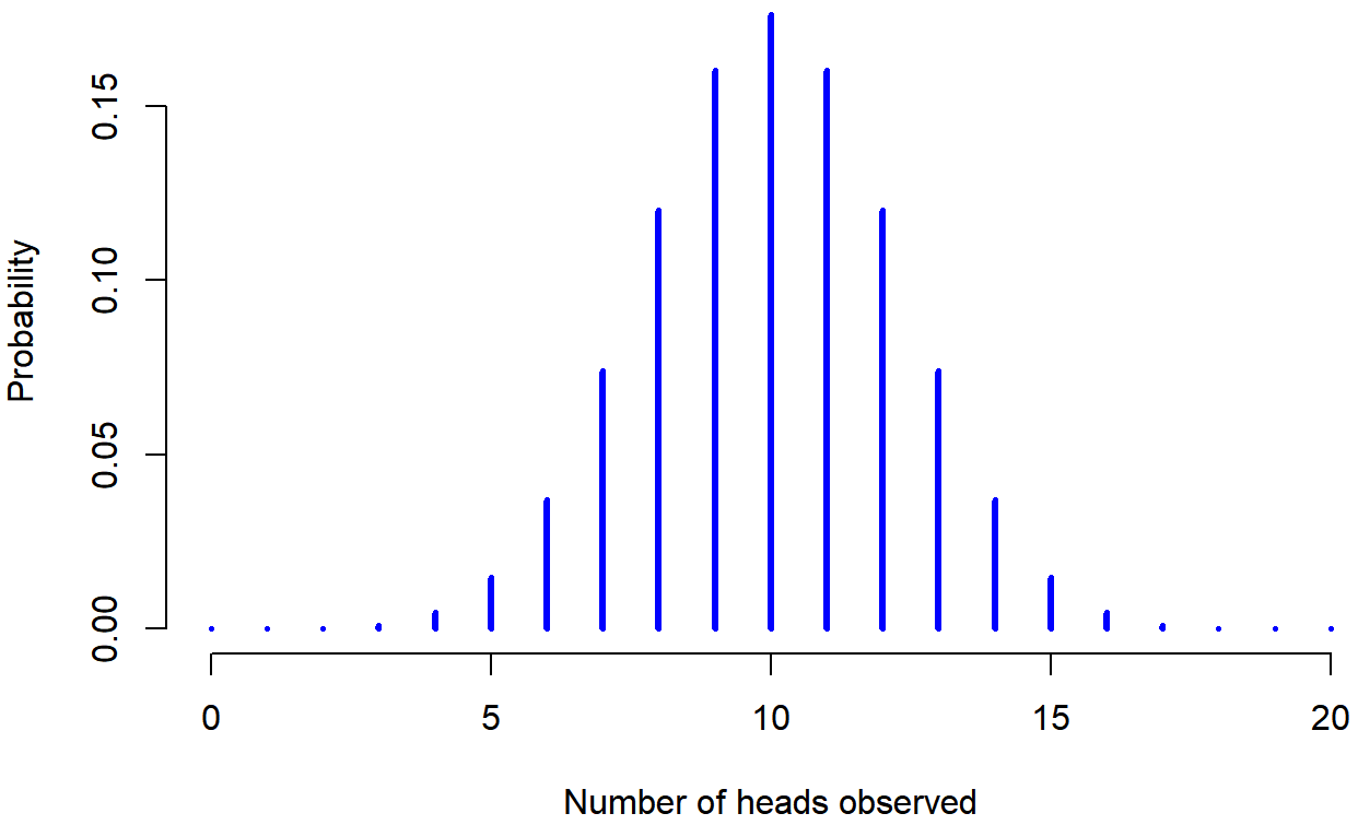
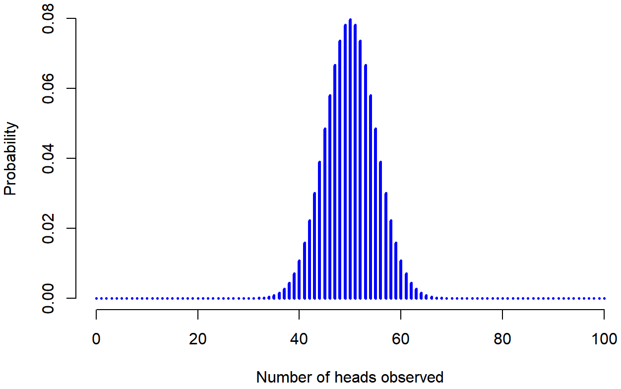
To give you a feel for how the binomial distribution changes when we alter the probability and N, let’s suppose that instead of rolling dice, I’m actually flipping coins. This time around, my experiment involves flipping a fair coin repeatedly, and the outcome that I’m interested in is the number of heads that I observe. In this scenario, the success probability is now 1/2 (one out of two options). Suppose I were to flip the coin N=20 times. In this example, I’ve changed the success probability (1 out of 2, instead of 1 out of 6 in the dice example), but kept the size of the experiment the same (N=20). What does this do to our binomial distribution? Well, as Figure \(\PageIndex{2}\) shows, the main effect of this is to shift the whole distribution higher (since there's more chance of getting a heads (one out of two options) than a 4 (one out of six options). Okay, what if we flipped a coin N=100 times? Well, in that case, we get Figure \(\PageIndex{3}\) . The distribution stays roughly in the middle, but there’s a bit more variability in the possible outcomes (meaning that there are more extreme scores); with more tosses, you are more likely to get no heads but also more likely to get all heads than if you only flipped the coin 20 times.

Figure \(\PageIndex{2}\)- Probability of Heads from Flipping a Fair Coin 20 Times (CC-BY-SA Danielle Navarro from Learning Statistics with R)

Figure \(\PageIndex{3}\)- Probability of Heads from Flipping a Fair Coin 100 Times (CC-BY-SA Danielle Navarro from Learning Statistics with R)
And that's it on binomial distributions! We are building understanding about distributions and sample size, so nothing too earth-shattering here. One thing to note is that both the coin flip and the dice toss were measured as discrete variables. Our next distributions will cover continuous variables. The difference is that discrete variables can be one or the other (a heads or a tails, a four or not-four), while continuous variables can have gradations shown as decimal points. Although the math works out to 3.33 skulls when you throw 30 dice, you can't actually get 3.33 skulls, you can only get 3 or 4 skulls.
We're building our knowledge, so keep going!


