3.1: Normal Distribution

Among all the distributions we see in practice, one is overwhelmingly the most common. The symmetric, unimodal, bell curve is ubiquitous throughout statistics. Indeed it is so common, that people often know it as the normal curve or normal distribution, shown in Figure \(\PageIndex{1}\). It is also known as the Gaussian distribution after Frederic Gauss, the first person to formalize its mathematical expression. Variables such as SAT scores and heights of US adult males closely follow the normal distribution.

Figure \(\PageIndex{1}\): A normal curve.

Many variables are nearly normal, but none are exactly normal. Thus the normal distribution, while not perfect for any single problem, is very useful for a variety of problems. We will use it in data exploration and to solve important problems in statistics.

Normal Distribution Model

The normal distribution model always describes a symmetric, unimodal, bell shaped curve. However, these curves can look different depending on the details of the model. Specifically, the normal distribution model can be adjusted using two parameters: mean and standard deviation. As you can probably guess, changing the mean shifts the bell curve to the left or right, while changing the standard deviation stretches or constricts the curve.

Figure \(\PageIndex{2}\): Both curves represent the normal distribution, however, they differ in their center and spread. The normal distribution with mean 0 and standard deviation 1 is called the standard normal distribution.

Figure \(\PageIndex{2}\) shows the normal distribution with mean 0 and standard deviation 1 in the left panel and the normal distributions with mean 19 and standard deviation 4 in the right panel. Figure \(\PageIndex{2}\) shows these distributions on the same axis.

Figure 3.2 but plotted together and on the same scale.

If a normal distribution has mean \(\mu\) and standard deviation \(\sigma\), we may write the distribution as \(N (\mu, \sigma)\). The two distributions in Figure \(\PageIndex{3}\) can be written as

\[N (\mu = 0, \sigma = 0)\]

and

\[N (\mu = 19, \sigma = 4).\]

Because the mean and standard deviation describe a normal distribution exactly, they are called the distribution's parameters.

Example \(\PageIndex{1}\)

Write down the short-hand for a normal distribution with

1. mean 5 and standard deviation 3,
2. mean -100 and standard deviation 10, and
3. mean 2 and standard deviation 9.

Solution

1. N(\(\mu\) = 5, \(\sigma\) = 3)
2. N(\(\mu\) = -100, \(\sigma\) = 10)
3. N(\(\mu\) = 2, \(\sigma\) = 9).

Standardizing with Z Scores

Example \(\PageIndex{2}\)

Table \(\PageIndex{1}\) shows the mean and standard deviation for total scores on the SAT and ACT. The distribution of SAT and ACT scores are both nearly normal. Suppose Ann scored 1800 on her SAT and Tom scored 24 on his ACT. Who performed better?

Table \(\PageIndex{1}\): Mean and standard deviation for the SAT and ACT.

	SAT	ACT
Mean	1500	21
SD	300	5

Solution

We use the standard deviation as a guide. Ann is 1 standard deviation above average on the SAT: 1500 + 300 = 1800. Tom is 0.6 standard deviations above the mean on the ACT: 21 + 0.6 X 5 = 24. In Figure \(\PageIndex{4}\), we can see that Ann tends to do better with respect to everyone else than Tom did, so her score was better.

Figure \(\PageIndex{4}\): Ann's and Tom's scores shown with the distributions of SAT and ACT scores.

Example \(\PageIndex{2}\) used a standardization technique called a Z score, a method most commonly employed for nearly normal observations but that may be used with any distribution. The Z score of an observation Z is defined as the number of standard deviations it falls above or below the mean. If the observation is one standard deviation above the mean, its Z score is 1. If it is 1.5 standard deviations below the mean, then its Z score is -1.5.

Definition: The Z score

The Z score of an observation is the number of standard deviations it falls above or below the mean. We compute the Z score for an observation \(x\) that follows a distribution with mean \(\mu\) and standard deviation \(\sigma\) using

\[Z = \dfrac {x - \mu}{\sigma}\]

Using \(\mu_{SAT}\) = 1500, \(\sigma_{SAT}\) = 300, and \(x_{Ann}\) = 1800, we find Ann's Z score in Example \(\PageIndex{2}\):

\[Z_{Ann} = \dfrac {x_{Ann} - \sigma_{SAT}}{\mu_{SAT}} = \dfrac {1800 - 1500}{300} = 1 \nonumber\]

Exercise \(\PageIndex{1}\)

Use Tom's ACT score, 24, along with the ACT mean and standard deviation to compute his Z score.

Answer

\(Z_{Tom} = \dfrac {x_{Tom} - \mu_{ACT}}{\sigma_{ACT}} = \dfrac {24 - 21}{5} = 0.6\)

Observations above the mean always have positive Z scores while those below the mean have negative Z scores. If an observation is equal to the mean (e.g. SAT score of 1500 in Example \(\PageIndex{2}\)), then the Z score is 0.

Exercise \(\PageIndex{2}\)

Let X represent a random variable from N(\(\mu\) = 3; \(\sigma\) = 2), and suppose we observe x = 5:19.

1. Find the Z score of x.
2. Use the Z score to determine how many standard deviations above or below the mean x falls.

Answer a

Its Z score is given by \(Z = \dfrac {x - \mu}{\sigma} = \dfrac {5.19 - 3}{2} = \dfrac {2.19}{2} = 1.095\).

Answer b

The observation x is 1.095 standard deviations above the mean. We know it must be above the mean since Z is positive.

Exercise \(\PageIndex{3}\)

Head lengths of brushtail possums follow a nearly normal distribution with mean 92.6 mm and standard deviation 3.6 mm. Compute the Z scores for possums with head lengths of 95.4 mm and 85.8 mm.

Answer

For \(x_1 = 95:4 mm: Z_1 = \dfrac {x_1 - \mu}{\sigma} = \dfrac {95.4 - 92.6}{3.6} = 0.78\). For \(x_2 = 85:8 mm: Z_2 = \dfrac {85:8 - 92:6}{3:6} = -1:89\).

We can use Z scores to roughly identify which observations are more unusual than others. One observation \(x_1\) is said to be more unusual than another observation \(x_2\) if the absolute value of its Z score is larger than the absolute value of the other observation's Z score: \(|Z_1| > |Z_2|\). This technique is especially insightful when a distribution is symmetric.

Exercise \(\PageIndex{4}\)

Which of the observations in Exercise \(\PageIndex{3}\) is more unusual?

Answer

Because the absolute value of Z score for the second observation is larger than that of the first, the second observation has a more unusual head length.

Normal Probability Table

Example \(\PageIndex{4}\):

Ann from Example \(\PageIndex{2}\) earned a score of 1800 on her SAT with a corresponding Z = 1. She would like to know what percentile she falls in among all SAT test-takers.

Solution

Ann's percentile is the percentage of people who earned a lower SAT score than Ann. We shade the area representing those individuals in Figure \(\PageIndex{5}\). The total area under the normal curve is always equal to 1, and the proportion of people who scored below Ann on the SAT is equal to the area shaded in Figure \(\PageIndex{5}\): 0.8413. In other words, Ann is in the 84th percentile of SAT takers.

Figure \(\PageIndex{5}\): The normal model for SAT scores, shading the area of those individuals who scored below Ann.

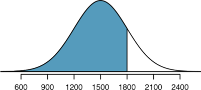
We can use the normal model to find percentiles. A normal probability table, which lists Z scores and corresponding percentiles, can be used to identify a percentile based on the Z score (and vice versa). Statistical software can also be used,

Figure \(\PageIndex{6}\): The area to the left of Z represents the percentile of the observation.

A normal probability table is given in Appendix B.1 on page 407 and abbreviated in Table 3.8. We use this table to identify the percentile corresponding to any particular Z score. For instance, the percentile of Z = 0:43 is shown in row 0:4 and column 0:03 in Table 3.8: 0.6664, or the 66:64th percentile. Generally, we round Z to two decimals, identify the proper row in the normal probability table up through the first decimal, and then determine the column representing the second decimal value. The intersection of this row and column is the percentile of the observation.

We can also find the Z score associated with a percentile. For example, to identify Z for the 80th percentile, we look for the value closest to 0.8000 in the middle portion of the table: 0.7995. We determine the Z score for the 80th percentile by combining the row and column Z values: 0.84.

Exercise \(\PageIndex{5}\)

Determine the proportion of SAT test takers who scored better than Ann on the SAT.

Answer

If 84% had lower scores than Ann, the number of people who had better scores must be 16%. (Generally ties are ignored when the normal model, or any other continuous distribution, is used.)

Normal Probability Examples

Cumulative SAT scores are approximated well by a normal model, \(N(\mu = 1500; \sigma = 300)\).

Example \(\PageIndex{5}\)

Shannon is a randomly selected SAT taker, and nothing is known about Shannon's SAT aptitude. What is the probability Shannon scores at least 1630 on her SATs?

Solution

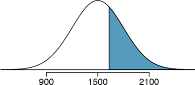
First, always draw and label a picture of the normal distribution. (Drawings need not be exact to be useful.) We are interested in the chance she scores above 1630, so we shade this upper tail:

Table \(\PageIndex{1}\): A section of the normal probability table. The percentile for a normal random variable with Z = 0.43 has been highlighted, and the percentile closest to 0.8000 has also been highlighted.

	Second decimal place of Z
Z	0.00	0.01	0.02	0.03	0.04	0.05	0.06	0.07	0.08	0.09
0.0	0.5000	0.5040	0.5080	0.5120	0.5160	0.5199	0.5239	0.5279	0.5319	0.5359
0.1	0.5398	0.5438	0.5478	0.5517	0.5557	0.5596	0.5636	0.5675	0.5714	0.5753
0.2	0.5793	0.5832	0.5871	0.5910	0.5948	0.5987	0.6026	0.6064	0.6103	0.6141
0.3	0.6179	0.6217	0.6255	0.6293	0.6331	0.6368	0.6406	0.6443	0.6480	0.6517
0.4	0.6554	0.6591	0.6628	0.6664	0.6700	0.6736	0.6772	0.6808	0.6844	0.6879
0.5	0.6915	0.6950	0.6985	0.7019	0.7054	0.7088	0.7123	0.7157	0.7190	0.7224
0.6	0.7257	0.7291	0.7324	0.7357	0.7389	0.7422	0.7454	0.7486	0.7517	0.7549
0.7	0.7580	0.7611	0.7642	0.7673	0.7704	0.7734	0.7764	0.7794	0.7823	0.7852
0.8	0.7881	0.7910	0.7939	0.7967	0.7995	0.8023	0.8051	0.8078	0.8106	0.8133
0.9	0.8159	0.8186	0.8212	0.8238	0.8264	0.8289	0.8315	0.8340	0.8365	0.8389
1.0	0.8413	0.8438	0.8461	0.8485	0.8508	0.8531	0.8554	0.8577	0.8599	0.8621
1.1	0.8643	0.8665	0.8686	0.8708	0.8729	0.8749	0.8770	0.8790	0.8810	0.8830
\(\vdots\)					\(\vdots\)

The picture shows the mean and the values at 2 standard deviations above and below the mean. The simplest way to find the shaded area under the curve makes use of the Z score of the cutoff value. With \(\mu\) = 1500, \(\sigma\) = 300, and the cutoff value x = 1630, the Z score is computed as

\[ Z = \dfrac {x - \mu}{\sigma} = \dfrac {1630 - 1500}{300} = \dfrac{130}{300} = 0.43\]

We look up the percentile of Z = 0:43 in the normal probability table shown in Table 3.8 or in Appendix B.1 on page 407, which yields 0.6664. However, the percentile describes those who had a Z score lower than 0.43. To find the area above Z = 0.43, we compute one minus the area of the lower tail:

The probability Shannon scores at least 1630 on the SAT is 0.3336.

TIP: always draw a picture first and find the Z score second

For any normal probability situation, always always always draw and label the normal curve and shade the area of interest first. The picture will provide an estimate of the probability. After drawing a figure to represent the situation, identify the Z score for the observation of interest.

Exercise \(\PageIndex{5}\)

If the probability of Shannon scoring at least 1630 is 0.3336, then what is the probability she scores less than 1630? Draw the normal curve representing this exercise, shading the lower region instead of the upper one.

Answer

We found the probability in Example \(\PageIndex{5}\): 0.6664. A picture for this exercise is represented by the shaded area below "0.6664" in Example 3.9.

Example \(\PageIndex{6}\)

Edward earned a 1400 on his SAT. What is his percentile?

Solution

First, a picture is needed. Edward's percentile is the proportion of people who do not get as high as a 1400. These are the scores to the left of 1400.

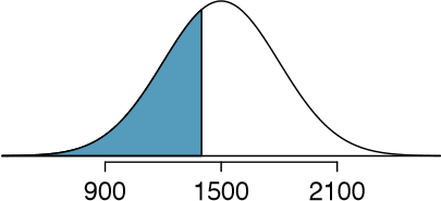
Identifying the mean \(\mu\) = 1500, the standard deviation \(\sigma\) = 300, and the cutoff for the tail area x = 1400 makes it easy to compute the Z score:

\[ Z = \dfrac {x - \mu}{\sigma} = \dfrac {1400 - 1500}{300} = - 0.33 \nonumber\]

Using the normal probability table, identify the row of -0.3 and column of 0.03, which corresponds to the probability 0.3707. Edward is at the 37th percentile.

Exercise \(\PageIndex{6A}\)

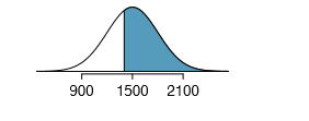
Use the results of Example \(\PageIndex{6}\) to compute the proportion of SAT takers who did better than Edward. Also draw a new picture.

Answer

If Edward did better than 37% of SAT takers, then about 63% must have done better than him.

TIP: areas to the right

The normal probability table in most books gives the area to the left. If you would like the area to the right, first find the area to the left and then subtract this amount from one.

Exercise \(\PageIndex{6b}\)

Stuart earned an SAT score of 2100. Draw a picture for each part.

1. What is his percentile?
2. What percent of SAT takers did better than Stuart?

Answer

TBA

Exercise \(\PageIndex{6C}\)

Based on a sample of 100 men, (USDA Food Commodity Intake Database) the heights of male adults between the ages 20 and 62 in the US is nearly normal with mean 70.0" and standard deviation 3.3". Mike is 5'7" and Jim is 6'4".

1. What is Mike's height percentile?
2. What is Jim's height percentile? Also draw one picture for each part.

Answer

First put the heights into inches: 67 and 76 inches. Figures are shown below. (a) \(Z_{Mike} = \dfrac {67-70}{3.3} = -0.91 \rightarrow 0.1814\). (b)\( Z_{Jim} = \dfrac {76-70}{3.3} = 1.82 \rightarrow 0.9656\)

The last several problems have focused on finding the probability or percentile for a particular observation. What if you would like to know the observation corresponding to a particular percentile?

Example \(\PageIndex{7}\):

Based on a sample of 100 men, (USDA Food Commodity Intake Database) the heights of male adults between the ages 20 and 62 in the US is nearly normal with mean 70.0" and standard deviation 3.3". Erik's height is at the 40th percentile. How tall is she?

Solution

As always, first draw the picture.

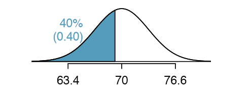
In this case, the lower tail probability is known (0.40), which can be shaded on the diagram. We want to find the observation that corresponds to this value. As a first step in this direction, we determine the Z score associated with the 40th percentile. Because the percentile is below 50%, we know Z will be negative. Looking in the negative part of the normal probability table, we search for the probability inside the table closest to 0.4000. We find that 0.4000 falls in row -0.2 and between columns 0.05 and 0.06. Since it falls closer to 0.05, we take this one: Z = -0.25.

Knowing \(Z_{Erik} = -0.25\) and the population parameters \(\mu\) = 70 and \(\sigma\) = 3.3 inches, the Z score formula can be set up to determine Erik's unknown height, labeled \(x_{Erik}\):

\[-0.25 = Z_{Erik} = \dfrac {x_{Erik} - \mu}{\sigma} = \dfrac {x_{Erik} - 70}{3.3}\]

Solving for \(x_{Erik}\) yields the height 69.18 inches. That is, Erik is about 5'9" (this is notation for 5-feet, 9-inches).

Exercise \(\PageIndex{7}\)

1. What is the 95th percentile for SAT scores?
2. What is the 97.5th percentile of the male heights?

As always with normal probability problems, first draw a picture.

Answer

Remember: draw a picture first, then find the Z score. (We leave the pictures to you.) The Z score can be found by using the percentiles and the normal probability table. (a) We look for 0.95 in the probability portion (middle part) of the normal probability table, which leads us to row 1.6 and (about) column 0.05, i.e. \(Z_{95} = 1.65. Knowing Z_{95} = 1.65, \mu = 1500, and \sigma = 300\), we setup the Z score formula: \(1.65 = \dfrac {x_{95} -1500}{300}\). We solve for \(x_{95}: x_{95} = 1995\). (b) Similarly, we find \(Z_{97:5} = 1.96\), again setup the Z score formula for the heights, and calculate \(x_{97.5} = 76.5\).

Example \(\PageIndex{8}\):

Based on a sample of 100 men, (USDA Food Commodity Intake Database) the heights of male adults between the ages 20 and 62 in the US is nearly normal with mean 70.0" and standard deviation 3.3". What is the adult male height at the 82nd percentile?

Solution

Again, we draw the figure first.

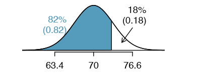
Next, we want to find the Z score at the 82nd percentile, which will be a positive value. Looking in the Z table, we find Z falls in row 0:9 and the nearest column is 0.02, i.e. Z = 0.92. Finally, the height x is found using the Z score formula with the known mean \(\mu\), standard deviation \(\sigma\), and Z score Z = 0.92:

\[ 0.92 = Z = \dfrac {x -\mu}{\sigma} = \dfrac {x - 70}{3.3} \nonumber\]

This yields 73.04 inches or about 6'1" as the height at the 82nd percentile.

Exercise \(\PageIndex{8}\)

Based on a sample of 100 men, (USDA Food Commodity Intake Database) the heights of male adults between the ages 20 and 62 in the US is nearly normal with mean 70.0" and standard deviation 3.3".

1. What is the probability that a randomly selected male adult is at least 6'2" (74 inches)?
2. What is the probability that a male adult is shorter than 5'9" (69 inches)?

Answer

Numerical answers: (a) 0.1131. (b) 0.3821.

Example \(\PageIndex{9}\):

Based on a sample of 100 men, (USDA Food Commodity Intake Database) the heights of male adults between the ages 20 and 62 in the US is nearly normal with mean 70.0" and standard deviation 3.3". What is the probability that a random adult male is between 5'9" and 6'2"?

Solution

These heights correspond to 69 inches and 74 inches. First, draw the figure. The area of interest is no longer an upper or lower tail.

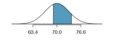
The total area under the curve is 1. If we find the area of the two tails that are not shaded (from Exercise 3.18, these areas are 0.3821 and 0.1131), then we can find the middle area:

That is, the probability of being between 5'9" and 6'2" is 0.5048.

Exercise \(\PageIndex{9A}\)

What percent of SAT takers get between 1500 and 2000?

Answer

This is an abbreviated solution. (Be sure to draw a figure!) First find the percent who get below 1500 and the percent that get above 2000: \(Z_{1500} = 0:00 \rightarrow 0.5000\) (area below), \(Z_{2000} = 1.67 \rightarrow 0.0475\) (area above). Final answer: 1:0000 - 0:5000 - 0.0475 = 0.4525.

Exercise \(\PageIndex{9B}\)

What percent of adult males are between 5'5" and 5'7"?

Answer

5'5" is 65 inches. 5'7" is 67 inches. Numerical solution: 1.000-0.0649-0.8183 = 0.1168, i.e. 11.68%.

68-95-99.7 Rule

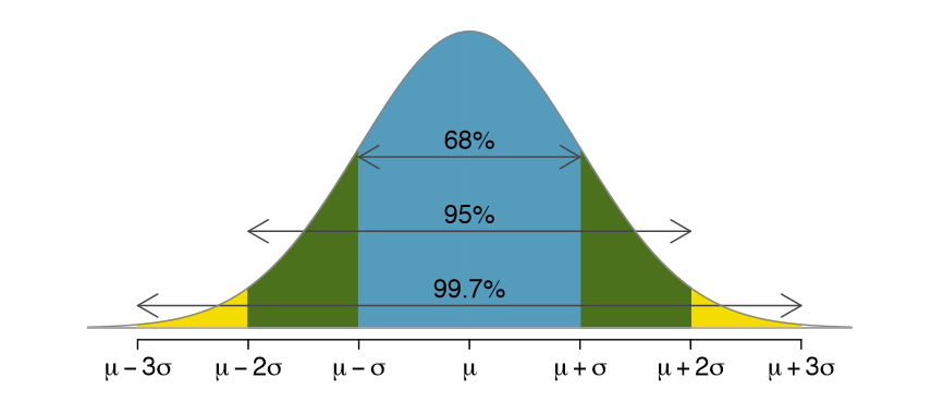
Here, we present a useful rule of thumb for the probability of falling within 1, 2, and 3 standard deviations of the mean in the normal distribution. This will be useful in a wide range of practical settings, especially when trying to make a quick estimate without a calculator or Z table.

Figure 3.9: Probabilities for falling within 1, 2, and 3 standard deviations of the mean in a normal distribution.

Exercise \(\PageIndex{10A}\)

Use the Z table to con rm that about 68%, 95%, and 99.7% of observations fall within 1, 2, and 3, standard deviations of the mean in the normal distribution, respectively. For instance, first find the area that falls between Z = -1 and Z = 1, which should have an area of about 0.68. Similarly there should be an area of about 0.95 between Z = -2 and Z = 2.

Answer

First draw the pictures. To nd the area between Z = -1 and Z = 1, use the normal probability table to determine the areas below Z = -1 and above Z = 1. Next verify the area between Z = -1 and Z = 1 is about 0.68. Repeat this for Z = -2 to Z = 2 and also for Z = -3 to Z = 3.

It is possible for a normal random variable to fall 4, 5, or even more standard deviations from the mean. However, these occurrences are very rare if the data are nearly normal. The probability of being further than 4 standard deviations from the mean is about 1-in-30,000. For 5 and 6 standard deviations, it is about 1-in-3.5 million and 1-in-1 billion, respectively.

Exercise \(\PageIndex{10B}\)

SAT scores closely follow the normal model with mean \(\mu\) = 1500 and standard deviation \(\sigma\) = 300. (a) About what percent of test takers score 900 to 2100? (b) What percent score between 1500 and 2100?

Answer

(a) 900 and 2100 represent two standard deviations above and below the mean, which means about 95% of test takers will score between 900 and 2100. (b) Since the normal model is symmetric, then half of the test takers from part (a) ( \(\frac {95%}{2} = 47:5% of all test takers) will score 900 to 1500 while 47.5% score between 1500 and 2100.

Contributors and Attributions

• David M Diez (Google/YouTube), Christopher D Barr (Harvard School of Public Health), Mine Çetinkaya-Rundel (Duke University)