
5.4: Power Calculations for a Difference of Means (Special Topic)
- Page ID
- 301

\( \newcommand{\vecs}[1]{\overset { \scriptstyle \rightharpoonup} {\mathbf{#1}} } \)
\( \newcommand{\vecd}[1]{\overset{-\!-\!\rightharpoonup}{\vphantom{a}\smash {#1}}} \)
\( \newcommand{\dsum}{\displaystyle\sum\limits} \)
\( \newcommand{\dint}{\displaystyle\int\limits} \)
\( \newcommand{\dlim}{\displaystyle\lim\limits} \)
\( \newcommand{\id}{\mathrm{id}}\) \( \newcommand{\Span}{\mathrm{span}}\)
( \newcommand{\kernel}{\mathrm{null}\,}\) \( \newcommand{\range}{\mathrm{range}\,}\)
\( \newcommand{\RealPart}{\mathrm{Re}}\) \( \newcommand{\ImaginaryPart}{\mathrm{Im}}\)
\( \newcommand{\Argument}{\mathrm{Arg}}\) \( \newcommand{\norm}[1]{\| #1 \|}\)
\( \newcommand{\inner}[2]{\langle #1, #2 \rangle}\)
\( \newcommand{\Span}{\mathrm{span}}\)
\( \newcommand{\id}{\mathrm{id}}\)
\( \newcommand{\Span}{\mathrm{span}}\)
\( \newcommand{\kernel}{\mathrm{null}\,}\)
\( \newcommand{\range}{\mathrm{range}\,}\)
\( \newcommand{\RealPart}{\mathrm{Re}}\)
\( \newcommand{\ImaginaryPart}{\mathrm{Im}}\)
\( \newcommand{\Argument}{\mathrm{Arg}}\)
\( \newcommand{\norm}[1]{\| #1 \|}\)
\( \newcommand{\inner}[2]{\langle #1, #2 \rangle}\)
\( \newcommand{\Span}{\mathrm{span}}\) \( \newcommand{\AA}{\unicode[.8,0]{x212B}}\)
\( \newcommand{\vectorA}[1]{\vec{#1}} % arrow\)
\( \newcommand{\vectorAt}[1]{\vec{\text{#1}}} % arrow\)
\( \newcommand{\vectorB}[1]{\overset { \scriptstyle \rightharpoonup} {\mathbf{#1}} } \)
\( \newcommand{\vectorC}[1]{\textbf{#1}} \)
\( \newcommand{\vectorD}[1]{\overrightarrow{#1}} \)
\( \newcommand{\vectorDt}[1]{\overrightarrow{\text{#1}}} \)
\( \newcommand{\vectE}[1]{\overset{-\!-\!\rightharpoonup}{\vphantom{a}\smash{\mathbf {#1}}}} \)
\( \newcommand{\vecs}[1]{\overset { \scriptstyle \rightharpoonup} {\mathbf{#1}} } \)
\(\newcommand{\longvect}{\overrightarrow}\)
\( \newcommand{\vecd}[1]{\overset{-\!-\!\rightharpoonup}{\vphantom{a}\smash {#1}}} \)
\(\newcommand{\avec}{\mathbf a}\) \(\newcommand{\bvec}{\mathbf b}\) \(\newcommand{\cvec}{\mathbf c}\) \(\newcommand{\dvec}{\mathbf d}\) \(\newcommand{\dtil}{\widetilde{\mathbf d}}\) \(\newcommand{\evec}{\mathbf e}\) \(\newcommand{\fvec}{\mathbf f}\) \(\newcommand{\nvec}{\mathbf n}\) \(\newcommand{\pvec}{\mathbf p}\) \(\newcommand{\qvec}{\mathbf q}\) \(\newcommand{\svec}{\mathbf s}\) \(\newcommand{\tvec}{\mathbf t}\) \(\newcommand{\uvec}{\mathbf u}\) \(\newcommand{\vvec}{\mathbf v}\) \(\newcommand{\wvec}{\mathbf w}\) \(\newcommand{\xvec}{\mathbf x}\) \(\newcommand{\yvec}{\mathbf y}\) \(\newcommand{\zvec}{\mathbf z}\) \(\newcommand{\rvec}{\mathbf r}\) \(\newcommand{\mvec}{\mathbf m}\) \(\newcommand{\zerovec}{\mathbf 0}\) \(\newcommand{\onevec}{\mathbf 1}\) \(\newcommand{\real}{\mathbb R}\) \(\newcommand{\twovec}[2]{\left[\begin{array}{r}#1 \\ #2 \end{array}\right]}\) \(\newcommand{\ctwovec}[2]{\left[\begin{array}{c}#1 \\ #2 \end{array}\right]}\) \(\newcommand{\threevec}[3]{\left[\begin{array}{r}#1 \\ #2 \\ #3 \end{array}\right]}\) \(\newcommand{\cthreevec}[3]{\left[\begin{array}{c}#1 \\ #2 \\ #3 \end{array}\right]}\) \(\newcommand{\fourvec}[4]{\left[\begin{array}{r}#1 \\ #2 \\ #3 \\ #4 \end{array}\right]}\) \(\newcommand{\cfourvec}[4]{\left[\begin{array}{c}#1 \\ #2 \\ #3 \\ #4 \end{array}\right]}\) \(\newcommand{\fivevec}[5]{\left[\begin{array}{r}#1 \\ #2 \\ #3 \\ #4 \\ #5 \\ \end{array}\right]}\) \(\newcommand{\cfivevec}[5]{\left[\begin{array}{c}#1 \\ #2 \\ #3 \\ #4 \\ #5 \\ \end{array}\right]}\) \(\newcommand{\mattwo}[4]{\left[\begin{array}{rr}#1 \amp #2 \\ #3 \amp #4 \\ \end{array}\right]}\) \(\newcommand{\laspan}[1]{\text{Span}\{#1\}}\) \(\newcommand{\bcal}{\cal B}\) \(\newcommand{\ccal}{\cal C}\) \(\newcommand{\scal}{\cal S}\) \(\newcommand{\wcal}{\cal W}\) \(\newcommand{\ecal}{\cal E}\) \(\newcommand{\coords}[2]{\left\{#1\right\}_{#2}}\) \(\newcommand{\gray}[1]{\color{gray}{#1}}\) \(\newcommand{\lgray}[1]{\color{lightgray}{#1}}\) \(\newcommand{\rank}{\operatorname{rank}}\) \(\newcommand{\row}{\text{Row}}\) \(\newcommand{\col}{\text{Col}}\) \(\renewcommand{\row}{\text{Row}}\) \(\newcommand{\nul}{\text{Nul}}\) \(\newcommand{\var}{\text{Var}}\) \(\newcommand{\corr}{\text{corr}}\) \(\newcommand{\len}[1]{\left|#1\right|}\) \(\newcommand{\bbar}{\overline{\bvec}}\) \(\newcommand{\bhat}{\widehat{\bvec}}\) \(\newcommand{\bperp}{\bvec^\perp}\) \(\newcommand{\xhat}{\widehat{\xvec}}\) \(\newcommand{\vhat}{\widehat{\vvec}}\) \(\newcommand{\uhat}{\widehat{\uvec}}\) \(\newcommand{\what}{\widehat{\wvec}}\) \(\newcommand{\Sighat}{\widehat{\Sigma}}\) \(\newcommand{\lt}{<}\) \(\newcommand{\gt}{>}\) \(\newcommand{\amp}{&}\) \(\definecolor{fillinmathshade}{gray}{0.9}\)It is also useful to be able to compare two means for small samples. For instance, a teacher might like to test the notion that two versions of an exam were equally difficult. She could do so by randomly assigning each version to students. If she found that the average scores on the exams were so different that we cannot write it off as chance, then she may want to award extra points to students who took the more difficult exam.
In a medical context, we might investigate whether embryonic stem cells can improve heart pumping capacity in individuals who have suffered a heart attack. We could look for evidence of greater heart health in the stem cell group against a control group.
In this section we use the t distribution for the difference in sample means. We will again drop the minimum sample size condition and instead impose a strong condition on the distribution of the data.
Sampling Distributions for the Difference in two Means
In the example of two exam versions, the teacher would like to evaluate whether there is convincing evidence that the difference in average scores between the two exams is not due to chance.
It will be useful to extend the t distribution method from Section 5.3 to apply to a difference of means:
\[\bar {x}_1 - \bar {x}_2\]
as a point estimate for
\[\mu _1 - \mu _2\]
Our procedure for checking conditions mirrors what we did for large samples in Section 5.2. First, we verify the small sample conditions (independence and nearly normal data) for each sample separately, then we verify that the samples are also independent. For instance, if the teacher believes students in her class are independent, the exam scores are nearly normal, and the students taking each version of the exam were independent, then we can use the t distribution for inference on the point estimate \(\bar {x}_1 - \bar {x}_2\).
The formula for the standard error of \(\bar {x}_1 - \bar {x}_2\)., introduced in Section 5.2, also applies to small samples:
\[ SE_{\bar {x}_1- \bar {x}_2} = \sqrt {SE^2_{\bar {x}_1} + SE^2_{\bar {x}_2}} = \sqrt { \dfrac {s^2_1}{n_1} +\dfrac {s^2_2}{n_2}} \tag {5.27}\]
19We use the row with 29 degrees of freedom. The value T = 2.39 falls between the third and fourth columns. Because we are looking for a single tail, this corresponds to a p-value between 0.01 and 0.025. The p-value is guaranteed to be less than 0.05 (the default signi cance level), so we reject the null hypothesis. The data provide convincing evidence to support the company's claim that student scores improve by more than 100 points following the class.
20This is an observational study, so we cannot make this causal conclusion. For instance, maybe SAT test takers tend to improve their score over time even if they don't take a special SAT class, or perhaps only the most motivated students take such SAT courses.
Because we will use the t distribution, we will need to identify the appropriate degrees of freedom. This can be done using computer software. An alternative technique is to use the smaller of \(n_1 - 1\) and \(n_2 - 1\), which is the method we will apply in the examples and exercises.21
Using the t distribution for a difference in means
The t distribution can be used for inference when working with the standardized difference of two means if (1) each sample meets the conditions for using the t distribution and (2) the samples are independent. We estimate the standard error of the difference of two means using Equation \ref{5.27}.
Two Sample t test
Summary statistics for each exam version are shown in Table 5.19. The teacher would like to evaluate whether this difference is so large that it provides convincing evidence that Version B was more difficult (on average) than Version A.
| Version | n | \(\bar {x}\) | s | min | max |
|---|---|---|---|---|---|
|
A B |
30 27 |
79.4 74.1 |
14 20 |
45 32 |
100 100 |
Exercise \(\PageIndex{1}\)
Construct a two-sided hypothesis test to evaluate whether the observed difference in sample means, \(\bar {x}_A - \bar {x}_B = 5.3\), might be due to chance.
Solution
Because the teacher did not expect one exam to be more difficult prior to examining the test results, she should use a two-sided hypothesis test. H0: the exams are equally difficult, on average. \(\mu_A - \mu_B = 0\). HA: one exam was more difficult than the other, on average. \(\mu_A - \mu_B \ne 0\).
Exercise \(\PageIndex{1}\)
To evaluate the hypotheses in Exercise 5.28 using the t distribution, we must first verify assumptions.
- Does it seem reasonable that the scores are independent within each group?
- What about the normality condition for each group?
- Do you think scores from the two groups would be independent of each other (i.e. the two samples are independent)?23
Solution
(a) It is probably reasonable to conclude the scores are independent.
(b) The summary statistics suggest the data are roughly symmetric about the mean, and it doesn't seem unreasonable to suggest the data might be normal. Note that since these samples are each nearing 30, moderate skew in the data would be acceptable.
(c) It seems reasonable to suppose that the samples are independent since the exams were handed out randomly.
After verifying the conditions for each sample and confirming the samples are independent of each other, we are ready to conduct the test using the t distribution. In this case, we are estimating the true difference in average test scores using the sample data, so the point estimate is \(\bar {x}_A - \bar {x}_B = 5.3\). The standard error of the estimate can be calculated using Equation \ref{5.27}:
\[ SE = \sqrt {\dfrac {s^2_A}{n_A} + \dfrac {s^2_B}{n_B}} = \sqrt {\dfrac {14^2}{30} + \dfrac {20^2}{27}} = 4.62\]
21This technique for degrees of freedom is conservative with respect to a Type 1 Error; it is more difficult to reject the null hypothesis using this df method.
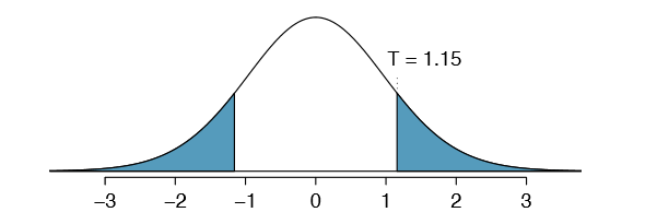
Figure 5.20: The t distribution with 26 degrees of freedom. The shaded right tail represents values with T \(\ge\) 1.15. Because it is a two-sided test, we also shade the corresponding lower tail.
Finally, we construct the test statistic:
\[T = \dfrac {\text {point estimate - null value}}{SE} = \dfrac {(79.4 - 74.1) - 0}{4.62} = 1.15\]
If we have a computer handy, we can identify the degrees of freedom as 45.97. Otherwise we use the smaller of \(n_1 - 1 \text {and} n_2 - 1\): df = 26.
Exercise \(\PageIndex{1}\)
Exercise 5.30 Identify the p-value, shown in Figure 5.20. Use df = 26.
Solution
We examine row df = 26 in the t table. Because this value is smaller than the value in the left column, the p-value is larger than 0.200 (two tails!). Because the p-value is so large, we do not reject the null hypothesis. That is, the data do not convincingly show that one exam version is more difficult than the other, and the teacher should not be convinced that she should add points to the Version B exam scores.
In Exercise 5.30, we could have used df = 45.97. However, this value is not listed in the table. In such cases, we use the next lower degrees of freedom (unless the computer also provides the p-value). For example, we could have used df = 45 but not df = 46.
Exercise \(\PageIndex{1}\)
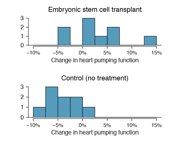
Do embryonic stem cells (ESCs) help improve heart function following a heart attack? Table 5.21 contains summary statistics for an experiment to test ESCs in sheep that had a heart attack. Each of these sheep was randomly assigned to the ESC or control group, and the change in their hearts' pumping capacity was measured. A positive value generally corresponds to increased pumping capacity, which suggests a stronger recovery.
- Set up hypotheses that will be used to test whether there is convincing evidence that ESCs actually increase the amount of blood the heart pumps.
- Check conditions for using the t distribution for inference with the point estimate \(\bar {x}_1 - \bar {x}_2\). To assist in this assessment, the data are presented in Figure 5.22.25
Solution
(a) We first setup the hypotheses:
- H0: The stem cells do not improve heart pumping function. \(\mu _{esc} - \mu _{control} = 0\).
- HA: The stem cells do improve heart pumping function. \(\mu _{esc} - \mu _{control} > 0\).
(b) Because the sheep were randomly assigned their treatment and, presumably, were kept separate from one another, the independence assumption is reasonable for each sample as well as for between samples. The data are very limited, so we can only check for obvious outliers in the raw data in Figure 5.22. Since the distributions are (very) roughly symmetric, we will assume the normality condition is acceptable. Because the conditions are satisfied, we can apply the t distribution.
| n | \(\bar {x}\) | s | |
|---|---|---|---|
|
ESCs control |
9 9 |
3.50 -4.33 |
5.17 2.76 |
Figure 5.23: Distribution of the sample difference of the test statistic if the null hypothesis was true. The shaded area, hardly visible in the right tail, represents the p-value.
Example \(\PageIndex{1}\)
Use the data from Table 5.21 and df = 8 to evaluate the hypotheses for the ESC experiment described in Exercise 5.31.
Solution
First, we compute the sample difference and the standard error for that point estimate:
\[\bar {x}_{esc} - \bar {x}_{control} = 7.88\]
\[SE = \dfrac {\dfrac {5.17^2}{9} + \dfrac {2.76^2}{9}} = 1.95\]
The p-value is depicted as the shaded slim right tail in Figure 5.23, and the test statistic is computed as follows:
\[T = \dfrac {7.88 - 0}{1.95} = 4.03\]
We use the smaller of \(n_1 - 1\) and \(n_2 - 1\) (each are the same) for the degrees of freedom: df = 8. Finally, we look for T = 4.03 in the t table; it falls to the right of the last column, so the p-value is smaller than 0.005 (one tail!). Because the p-value is less than 0.005 and therefore also smaller than 0.05, we reject the null hypothesis. The data provide convincing evidence that embryonic stem cells improve the heart's pumping function in sheep that have suffered a heart attack.
Two sample t confidence interval
The results from the previous section provided evidence that ESCs actually help improve the pumping function of the heart. But how large is this improvement? To answer this question, we can use a confidence interval.
Exercise \(\PageIndex{1}\)
In Exercise 5.31, you found that the point estimate, \(\bar {x}_{esc} - \bar {x}_{control} = 7.88\), has a standard error of 1.95. Using df = 8, create a 99% confidence interval for the improvement due to ESCs.
Solution
We know the point estimate, 7.88, and the standard error, 1.95. We also veri ed the conditions for using the t distribution in Exercise 5.31. Thus, we only need identify \(t*_8\) to create a 99% con dence interval: \(t*_8 = 3.36\). The 99% con dence interval for the improvement from ESCs is given by
\[\text {point estimate} \pm t*_8 SE \rightarrow 7.88 \pm 3.36 \times 1.95 \rightarrow (1.33, 14.43)\]
That is, we are 99% con dent that the true improvement in heart pumping function is somewhere between 1.33% and 14.43%.
Pooled Standard Deviation Estimate (special topic)
Occasionally, two populations will have standard deviations that are so similar that they can be treated as identical. For example, historical data or a well-understood biological mechanism may justify this strong assumption. In such cases, we can make our t distribution approach slightly more precise by using a pooled standard deviation. The pooled standard deviation of two groups is a way to use data from both samples to better estimate the standard deviation and standard error. If s1 and s2 are the standard deviations of groups 1 and 2 and there are good reasons to believe that the population standard deviations are equal, then we can obtain an improved estimate of the group variances by pooling their data:
\[s^2_{pooled} = \dfrac {s^2_1 \times (n_1 - 1) + s^2_2 \times (n_2 - 1)}{n_1 + n_2 - 2}\]
where \(n_1\) and \(n_2\) are the sample sizes, as before. To use this new statistic, we substitute \(s^2_{pooled}\) in place of \(s^2_1\) and \(s^2_2\) in the standard error formula, and we use an updated formula for the degrees of freedom:
\[df = n_1 + n_2 - 2\]
The bene ts of pooling the standard deviation are realized through obtaining a better estimate of the standard deviation for each group and using a larger degrees of freedom parameter for the t distribution. Both of these changes may permit a more accurate model of the sampling distribution of \(\bar {x}^2_1 - \bar {x}^2_2\)
Caution: Pooling standard deviations should be done only after careful research
A pooled standard deviation is only appropriate when background research indicates the population standard deviations are nearly equal. When the sample size is large and the condition may be adequately checked with data, the benefits of pooling the standard deviations greatly diminishes.