5.7: Putting it All Together

So, we've spend a lot of time going over different distributions. Why? Because they can answer research questions!

Standard Normal Curve

In Figure \(\PageIndex{1}\), the x-axis corresponds to the value of some variable, and the y-axis tells us something about how likely we are to observe that value.

Figure \(\PageIndex{1}\)- Standard Normal Curve (CC-BY-SA Danielle Navarro from Learning Statistics with R)

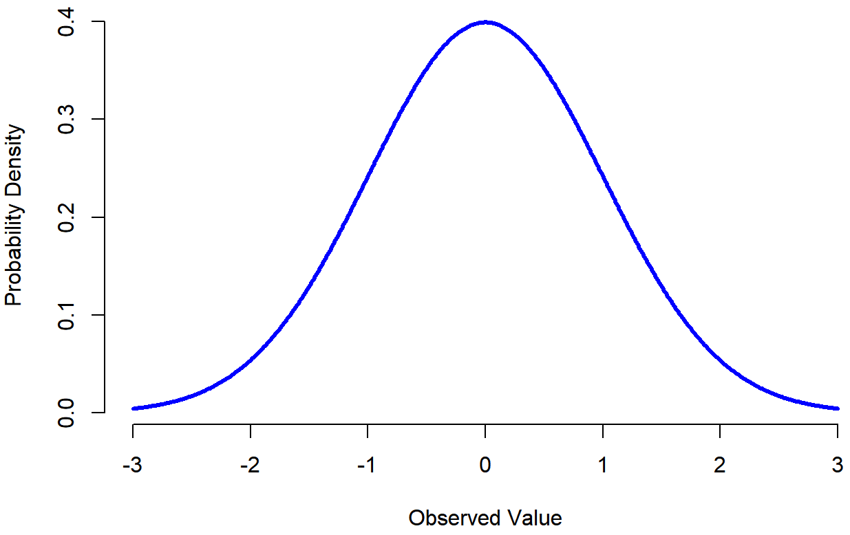
You can see where the name “bell curve” comes from in Figure \(\PageIndex{1}\) it looks a bit like a bell. Notice that, unlike the binomial distribution, the normal distribution in Figure \(\PageIndex{1}\) shows a smooth curve instead of “histogram-like” bars. This isn’t an arbitrary choice: the normal distribution is like a quantitative variable when the variable can be measured with decimals or fractions (called a continuous variable), whereas the binomial distribution is like a qualitative variable (called discrete variables). For instance, in the die rolling example, it was possible to get 3 skulls or 4 skulls, but impossible to get 3.9 skulls. Qualitative variables that are continuous don’t have this constraint. For instance, suppose we’re talking about the weather. The temperature on a pleasant spring day could be 68 degrees, 69.67 degrees, or even 72.222 degrees; temperature can be anything in between since temperature is a continuous variable, and so a normal distribution might be quite appropriate for describing Spring temperatures.

This is where it all comes together! What we can start doing with these distributions is comparing them. This might not sound like much, but it's the foundation of statistics, and allows us to answer research questions and test hypotheses.

• Probability Distributions: We know that we can make predictions from probability distributions. I can use probability distributions to understand the likelihood of specific events happening.
• Law of Large Numbers: We know through the Law of Large Numbers that with big enough samples, their scores will be normally distributed (with all of the important characteristics that includes).
• Central Limit Theorem: We know through the Central Limit Theorem that if we get the means of enough samples, that the sampling distribution of means will be normally distributed.
• Standard Normal Distributions: We know that the mean is converted to always be zero, and the standard deviation is standardized to always be 1 in Standard Normal Distributions. We also know that there are predictable portions of scores between the mean and standard deviation.

The last important piece is learning that a special feature of normal distributions is that we know the proportions (percentages) of cases that should (probability) fall within each standard deviation around the mean. Irrespective of what the actual mean and standard deviation are, 68.3% of the area falls within 1 standard deviation of the mean. Similarly, 95.4% of the distribution falls within 2 standard deviations of the mean, and 99.7% of the distribution is within 3 standard deviations. This idea is illustrated in the follow Figures.

Figure \(\PageIndex{2}\)- About 68% of Scores are One Standard Deviation Below through One Standard Deviation Above the Mean (CC-BY-SA Danielle Navarro from Learning Statistics with R)

Figure \(\PageIndex{3}\)- About 95% of Scores are Two Standard Deviations Below through Two Standard Deviations Above the Mean (CC-BY-SA Danielle Navarro from Learning Statistics with R)

Figure \(\PageIndex{4}\)- About 16% of Scores Should Be Less Than Two Standard Deviations Below the Mean (CC-BY-SA Danielle Navarro from Learning Statistics with R)

Figure \(\PageIndex{5}\)- About 34% of Scores Should Be One Standard Deviations Below the Mean (CC-BY-SA Danielle Navarro from Learning Statistics with R)

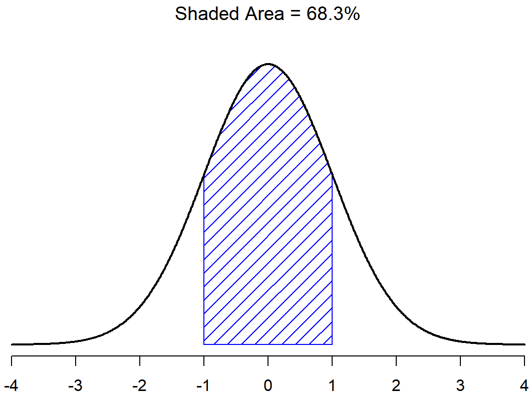
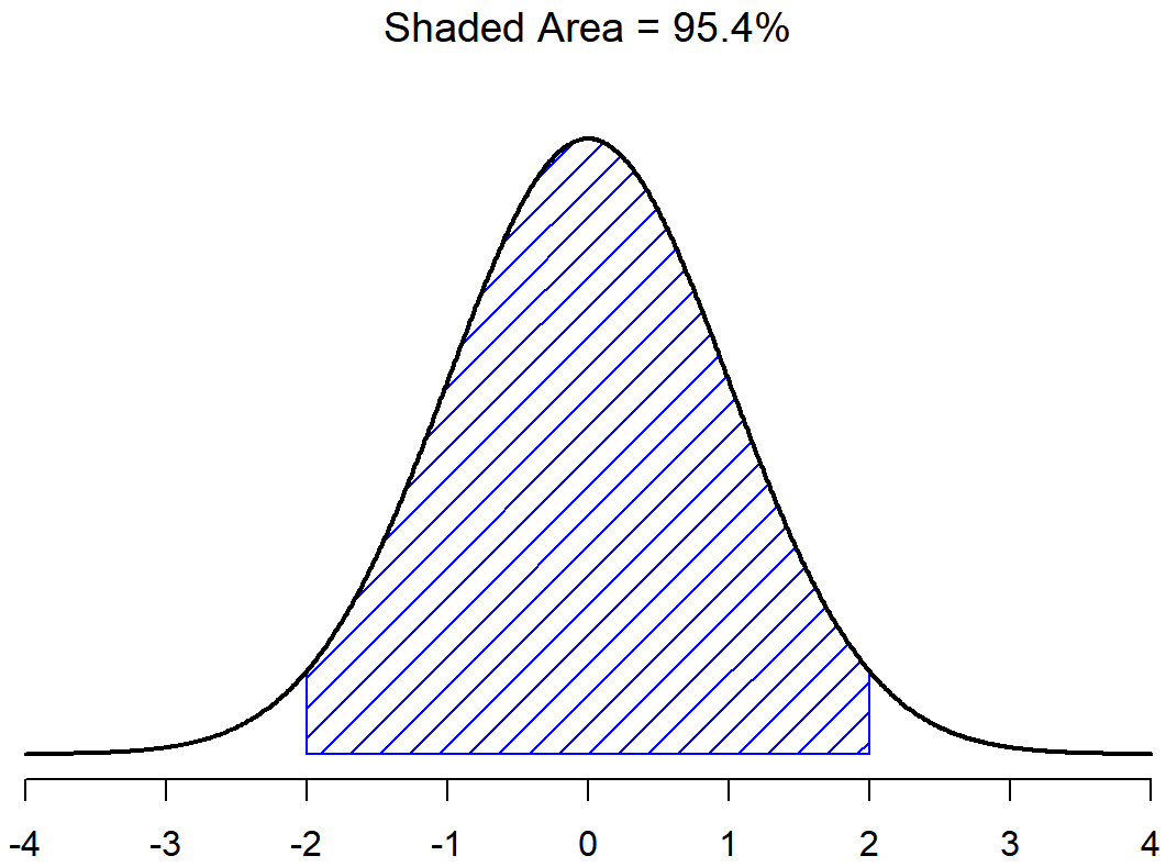
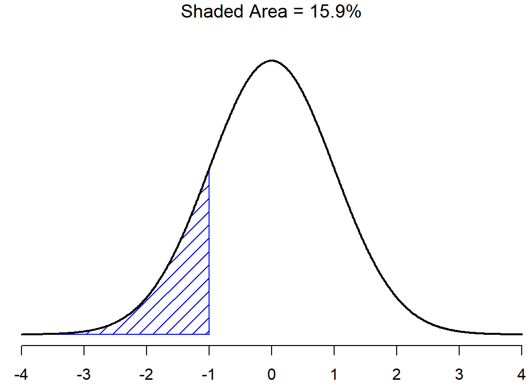
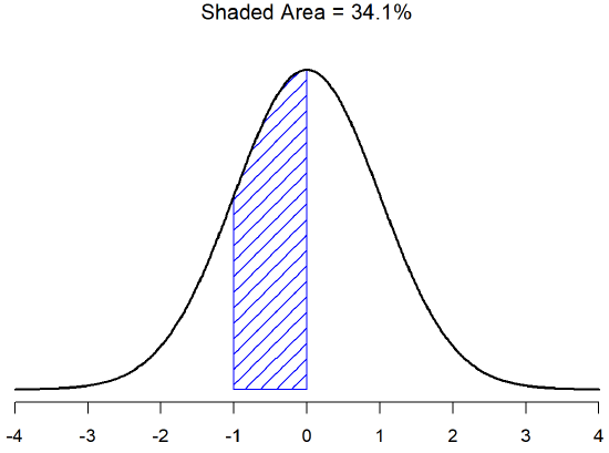
There is a 68.3% chance (probability) that a score from any sample will fall within the shaded area of Figure \(\PageIndex{2}\), and a 95.4% chance that an observation will fall within two standard deviations of the mean (the shaded area in Figure \(\PageIndex{3}\)). Similarly, there is a 15.9% chance that an observation will be below one standard deviation below the mean. There is a 34.1% chance that the observation is greater than one standard deviation below the mean but still below the mean (Figure \(\PageIndex{5}\)). Notice that if you add these two numbers together you get 15.9+34.1=50. For normally distributed data, there is a 50% chance that an observation falls below the mean. Of course that also implies that there is a 50% chance that it falls above the mean.

For the interest of simplicity, let’s round these percentages to whole numbers, as can be seen in (Figure \(\PageIndex{6}\)).

Figure \(\PageIndex{6}\): Empirical Rule. (CC-BY-SA; Dan Kernler from Wikipedia)

Figure \(\PageIndex{6}\) uses the symbols for a population; you’ve learned several ideas in this chapter that would explain why the Standard Normal Curve would have characteristics of the population! Let’s start with the inner lines. Figure \(\PageIndex{6}\) shows that 68% of the scores fall within one standard deviation around the mean. On the x-axis, you can see that this 68% includes one population mean (\(\mu\)) minus one population standard deviation (\(\sigma\)) as well as the mean plus one standard deviation. Figure \(\PageIndex{5}\) shows why this is the case: one standard deviation below the mean is about 34% of the whole distribution. As the Standard Normal Distribution is symmetrical, that means that one standard deviation above the means also should include about 34% of the scores. Adding those together (34% plus 34% = 68%). What Figure \(\PageIndex{6}\) illustrates is that we can predict the proportion of scores that should be one, two or three standard deviations around the mean for distributions that are normally distributed.

Because we know the proportion of scores that should be between the mean and each standard deviation, we can also predict the number of scores that we would expect to fall within that range for a new sample (if we knew the new sample size). Let’s practice a little to see how this could be useful.

Table \(\PageIndex{1}\)- Descriptive Statistics for Research Activity Points for Face-to-Face Class

Descriptive Statistic	Research Activities Points
N:	9
Mean:	68.78
Median:	64
Mode:	64
SD	10.78

We’ll discuss a set of data that we’ve already covered, the Research Activities points for a face-to-face section behavioral statistics (Table \(\PageIndex{1}\)). Everything that we’ve learned so far can be applied (again) to this data, so you could name the sample, such as “The sample is nine students in a face-to-face section of behavioral statistics.” Once you know the sample, you can name a possible population, such as “This sample can represent all face-to-face behavioral statistics sections.” As we previously did, you can use the measures of central tendency (and standard deviation) to predict the shape of the frequency distribution.

Based on these measures of central tendency and variability, do you think that this face-to-face section did well on their research activities, or not so much?

The research activities’ measures of central tendency are pretty low (the mean, median, and mode are all a D grade), and the standard deviation is medium, so I don’t think that the face-to-face class did too well on these research activities.

Let’s get to some new ways that we can apply this information!

Example \(\PageIndex{1}\)

1. What percentage of the Research Activities scores should be one standard deviation around the mean (one standard deviation below the mean and one standard deviation above the mean)?
2. What percentage of the Research Activities scores should be two standard deviations around the mean (two standard deviations below the mean and two standard deviations above the mean)?

Solution

You don’t have to do math! You can just look at Figure \(\PageIndex{6}\).

1. Looking at Figure \(\PageIndex{6}\)) 68% of scores should fall within one standard deviation around the mean.
2. Looking at Figure \(\PageIndex{6}\)) 95% of scores should fall within one standard deviation around the mean.

To use the properties of the Standard Normal Curve, we first figure out what scores are one standard deviation around the mean. To find the scores that mark one standard deviation around the mean, we conduct two calculations; we first find the score that is one standard deviation below the mean (which is \(\bar{X} + s \)) and then finding the score that is one standard deviation above the mean (\(\bar{X} + s \)).

Example \(\PageIndex{2}\)

1. What is the Research Activities score that is one standard deviation below the mean?
2. What is the Research Activities score that is one standard deviation above the mean?
3. What is the Research Activities score that is two standard deviations below the mean?
4. What is the Research Activities score that is two standard deviations above the mean?

Solution

1. The Research Activities score that is one standard deviation below the mean is 58.01 points because \(\bar{X} - s = 68.75-10.77 = 58.01 \).
2. The Research Activities score that is one standard deviation above the mean is 79.55 points because \(\bar{X} + s = 68.75+10.77 = 79.55 \).
3. The Research Activities score that is two standard deviations below the mean is 47.24 points. You can answer this in two mathematical ways:
   1. \(\bar{X} - s - s = 68.75-10.77-10.77 = 47.24 \)
   2. \(\bar{X} - 2s = 68.75 - (2 \times 10.77) = 68.75 - 21.54 = 47.24 \)
   3. These two formulas are mathematically identical, so choose the one that makes the most sense to you.
4. The Research Activities score that is two standard deviations above the mean is 90.32 points because
   1. \(\bar{X} + s + s = 68.75 +10.77 = 10.77 = 90.32 \)
   2. \(\bar{X} - 2s = 68.75 + (2 \times 10.77) = 68.75 + 21.54 = 90.32 \)

This means that one standard deviation around the mean for this face-to-face sample is 58.01 to 79.55 points, and two standard deviations around the mean would be Research Activities scores of 47.24 points to 90.32 points. Combining that with the proportions in the Standard Normal Curve (see Figure \(\PageIndex{6}\)), we can estimate the percentage of students who actually scored in these ranges.

In other words, we would predict (if our distribution of Research Activities scores was normally distributed) that 68% of scores for Research Activities would fall between 58.01 and 79.55, and that 95% of scores should fall between 47.24 points to 90.32 points. Just like when we used the measures of central tendency and standard deviation to predict the shape of a frequency distribution without looking at an actual frequency line graph, we can use the properties of the Standard Normal Distribution to get a sense of what the frequency line graph might look like.

We can add one more step to use this information to predict the actual number of students who would score one standard deviation around the mean for a new sample. For our example of Research Activities scores, this might be useful to estimate the number of students who would score a C or D on these assignments. Looking back at the example, we see that about 68% of scores should score between 58.01 and 79.55 points (which is almost a D to a C grade). If Dr. MO had a new class, we could figure out what 68% of that class would be:

\[\frac{68}{100} \times N \nonumber\]

This converts the percentage to a decimal, then multiplies that by the total number of scores in the new sample.

Example \(\PageIndex{3}\)

If Dr. MO used this information about the Research Activities scores from the face-to-face class of nine students, how many students should she expect to earn scores one standard deviation around the mean (near a D to a C grade) if she had a new class of 30 students?

Solution

\[\frac{68}{100} \times N = 0.68 \times 30 = 20.40 \nonumber\]

With a new class of 30 students, Dr. MO should expect about 20.40 students to score between 58.01 points to 79.55 points.

Unfortunately, our distribution was not normally distributed (see Figure \(\PageIndex{7}\)), so these estimates were incorrect. We didn’t do anything wrong mathematically or in our interpretation, though! It’s just that small sample sizes tend to not be normally distributed (as you could predict from the Law of Large Numbers), so the Standard Normal Distribution doesn’t apply well. This shows us that using the Standard Normal Curve to predict percentages is not guaranteed to be accurate.

Figure \(\PageIndex{7}\): Frequency Line Graph of Face-to-Face Class's Research Activities Scores. (CC-BY-SA Michelle Oja via personal records)

You might also have notice that you could have pretty easily used Figure \(\PageIndex{7}\)) (or the original raw data or frequency table) to just count scores that would be between the range of one standard deviation around the mean. For example, you could mark 58.01 and 79.55 on Figure \(\PageIndex{7}\)), and counted the number of scores that fall within your calculations of one standard deviation below and above the mean. This is totally valid! However, most researchers are working with hundreds of scores, sometimes even millions. You wouldn’t want to hand-count all of those scores! The ability to remember the proportion of scores that should fall one or two standard deviations around the mean, plus the math literacy to calculate the scores that mark these percentages, can lead to the statistical literacy to make predictions about the actual number of scores in any distribution of quantitative (continuous) data that you’re shown.

Note

When might it be useful in your future career to know the expected proportion or even the actual number, of clients you could expect to “score” one standard deviation around the mean?

Let’s go through the process one more time. We can use the information from Table \(\PageIndex{2}\), which describes the Research Activities scores for the online section that we analyzed previously.

You might want to make a flow chart or decision tree to help you follow the process before your statistical literacy is stronger.

Table \(\PageIndex{2}\)- Descriptive Statistics for Research Activity Points for Online Class

Descriptive Statistic	Research Activities Points
N:	12
Mean:	80.58
Median:	81
Mode:	88
SD	12.43

Again, everything that we’ve learned so far can be applied to the data set described in Table \(\PageIndex{2}\).

Exercise \(\PageIndex{1}\)

1. Who is the sample?
2. Who might be the population?

Answer

1. The sample is 12 students in an online section of behavioral statistics.
2. This sample could represent all online sections of behavioral statistics; this could be the population.

Exercise \(\PageIndex{2}\)

Based on these measures of central tendency and variability, do you think that this online section did well on their research activities, or not so much?

Answer

The research activities’ measures of central tendency are pretty good (the mean, median, and mode are all a B grade), and the standard deviation is medium, so I think that the online class did pretty well on these research activities.

Before we get too far, let’s remind ourselves of the proportions in a Standard Normal Curve.

Exercise \(\PageIndex{3}\)

1. What percentage of the Research Activities scores should be one standard deviation around the mean (one standard deviation below the mean and one standard deviation above the mean)?
2. What percentage of the Research Activities scores should be two standard deviations around the mean (two standard deviations below the mean and two standard deviations above the mean)?

Answer

1. Looking at Figure \(\PageIndex{6}\)) 68% of scores should fall within one standard deviation around the mean.
2. Looking at Figure \(\PageIndex{6}\)) 95% of scores should fall within one standard deviation around the mean.

Exercise \(\PageIndex{4}\)

1. What is the Research Activities score that is one standard deviation below the mean?
2. What is the Research Activities score that is one standard deviation above the mean?

Answer

1. The Research Activities score that is one standard deviation below the mean is 68.15 points because \(\bar{X} - s = 80.58-12.43 = 68.15 \).
2. The Research Activities score that is one standard deviation above the mean is 79.55 points because \(\bar{X} + s = 80.58+12.43 = 93.01 \).

This means that one standard deviation around the mean for this online section is 68.15 to 93.01 points. Combining that with the proportions in the Standard Normal Curve (see Figure \(\PageIndex{6}\)), we can estimate the percentage of students who actually scored in these ranges: we predict (if our distribution of Research Activities scores was normally distributed) that 68% of scores for Research Activities would fall between 68.15 points and 93.01 points. Without looking at an actual frequency line graph, we could get a sense that this section did pretty well since 68% got close to a C up to an A grade.

Adding one more step, let’s predict the number of students who we would expect to score in this range (one standard deviation around the mean) in a new sample of online students in a behavioral statistics course.

Exercise \(\PageIndex{5}\)

If Dr. MO used this information on the Research Activities scores from the online class, how many students should she expect to earn scores one standard deviation around the mean if she had a new class of 25 students?

Answer

\[\frac{68}{100} \times N = 0.68 \times 25 = 17.00 \nonumber\]

With a new class of 30 students, Dr. MO should expect about 17 students to score between 68.15 points to 93.01 points

Add texts here. Do not delete this text first.

Summary

The ideas in this chapter are the foundation for statistical analyses and statistical hypothesis testing. Don’t worry too much if this chapter didn’t make sense. You can still learn everything in the rest of this textbook even if you haven’t put these pieces in the puzzle yet. Just keep working! For some people, you have to see the big picture (which come up in the chapters when we finally test research hypotheses) before these pieces about distributions fits into the picture. As you continue to work with data, your statistical literacy will improve. Eventually, if you keep analyzing data to answer questions, these big ideas will make sense! But in the meantime, you can still analyze and interpret the data that we’ll be working with.

Contributors and Attributions

• Danielle Navarro (University of New South Wales)

• Dr. MO (Taft College)