11.3: Goodness-of-Fit (1 of 2)
- Page ID
- 14193
\( \newcommand{\vecs}[1]{\overset { \scriptstyle \rightharpoonup} {\mathbf{#1}} } \)
\( \newcommand{\vecd}[1]{\overset{-\!-\!\rightharpoonup}{\vphantom{a}\smash {#1}}} \)
\( \newcommand{\id}{\mathrm{id}}\) \( \newcommand{\Span}{\mathrm{span}}\)
( \newcommand{\kernel}{\mathrm{null}\,}\) \( \newcommand{\range}{\mathrm{range}\,}\)
\( \newcommand{\RealPart}{\mathrm{Re}}\) \( \newcommand{\ImaginaryPart}{\mathrm{Im}}\)
\( \newcommand{\Argument}{\mathrm{Arg}}\) \( \newcommand{\norm}[1]{\| #1 \|}\)
\( \newcommand{\inner}[2]{\langle #1, #2 \rangle}\)
\( \newcommand{\Span}{\mathrm{span}}\)
\( \newcommand{\id}{\mathrm{id}}\)
\( \newcommand{\Span}{\mathrm{span}}\)
\( \newcommand{\kernel}{\mathrm{null}\,}\)
\( \newcommand{\range}{\mathrm{range}\,}\)
\( \newcommand{\RealPart}{\mathrm{Re}}\)
\( \newcommand{\ImaginaryPart}{\mathrm{Im}}\)
\( \newcommand{\Argument}{\mathrm{Arg}}\)
\( \newcommand{\norm}[1]{\| #1 \|}\)
\( \newcommand{\inner}[2]{\langle #1, #2 \rangle}\)
\( \newcommand{\Span}{\mathrm{span}}\) \( \newcommand{\AA}{\unicode[.8,0]{x212B}}\)
\( \newcommand{\vectorA}[1]{\vec{#1}} % arrow\)
\( \newcommand{\vectorAt}[1]{\vec{\text{#1}}} % arrow\)
\( \newcommand{\vectorB}[1]{\overset { \scriptstyle \rightharpoonup} {\mathbf{#1}} } \)
\( \newcommand{\vectorC}[1]{\textbf{#1}} \)
\( \newcommand{\vectorD}[1]{\overrightarrow{#1}} \)
\( \newcommand{\vectorDt}[1]{\overrightarrow{\text{#1}}} \)
\( \newcommand{\vectE}[1]{\overset{-\!-\!\rightharpoonup}{\vphantom{a}\smash{\mathbf {#1}}}} \)
\( \newcommand{\vecs}[1]{\overset { \scriptstyle \rightharpoonup} {\mathbf{#1}} } \)
\( \newcommand{\vecd}[1]{\overset{-\!-\!\rightharpoonup}{\vphantom{a}\smash {#1}}} \)
\(\newcommand{\avec}{\mathbf a}\) \(\newcommand{\bvec}{\mathbf b}\) \(\newcommand{\cvec}{\mathbf c}\) \(\newcommand{\dvec}{\mathbf d}\) \(\newcommand{\dtil}{\widetilde{\mathbf d}}\) \(\newcommand{\evec}{\mathbf e}\) \(\newcommand{\fvec}{\mathbf f}\) \(\newcommand{\nvec}{\mathbf n}\) \(\newcommand{\pvec}{\mathbf p}\) \(\newcommand{\qvec}{\mathbf q}\) \(\newcommand{\svec}{\mathbf s}\) \(\newcommand{\tvec}{\mathbf t}\) \(\newcommand{\uvec}{\mathbf u}\) \(\newcommand{\vvec}{\mathbf v}\) \(\newcommand{\wvec}{\mathbf w}\) \(\newcommand{\xvec}{\mathbf x}\) \(\newcommand{\yvec}{\mathbf y}\) \(\newcommand{\zvec}{\mathbf z}\) \(\newcommand{\rvec}{\mathbf r}\) \(\newcommand{\mvec}{\mathbf m}\) \(\newcommand{\zerovec}{\mathbf 0}\) \(\newcommand{\onevec}{\mathbf 1}\) \(\newcommand{\real}{\mathbb R}\) \(\newcommand{\twovec}[2]{\left[\begin{array}{r}#1 \\ #2 \end{array}\right]}\) \(\newcommand{\ctwovec}[2]{\left[\begin{array}{c}#1 \\ #2 \end{array}\right]}\) \(\newcommand{\threevec}[3]{\left[\begin{array}{r}#1 \\ #2 \\ #3 \end{array}\right]}\) \(\newcommand{\cthreevec}[3]{\left[\begin{array}{c}#1 \\ #2 \\ #3 \end{array}\right]}\) \(\newcommand{\fourvec}[4]{\left[\begin{array}{r}#1 \\ #2 \\ #3 \\ #4 \end{array}\right]}\) \(\newcommand{\cfourvec}[4]{\left[\begin{array}{c}#1 \\ #2 \\ #3 \\ #4 \end{array}\right]}\) \(\newcommand{\fivevec}[5]{\left[\begin{array}{r}#1 \\ #2 \\ #3 \\ #4 \\ #5 \\ \end{array}\right]}\) \(\newcommand{\cfivevec}[5]{\left[\begin{array}{c}#1 \\ #2 \\ #3 \\ #4 \\ #5 \\ \end{array}\right]}\) \(\newcommand{\mattwo}[4]{\left[\begin{array}{rr}#1 \amp #2 \\ #3 \amp #4 \\ \end{array}\right]}\) \(\newcommand{\laspan}[1]{\text{Span}\{#1\}}\) \(\newcommand{\bcal}{\cal B}\) \(\newcommand{\ccal}{\cal C}\) \(\newcommand{\scal}{\cal S}\) \(\newcommand{\wcal}{\cal W}\) \(\newcommand{\ecal}{\cal E}\) \(\newcommand{\coords}[2]{\left\{#1\right\}_{#2}}\) \(\newcommand{\gray}[1]{\color{gray}{#1}}\) \(\newcommand{\lgray}[1]{\color{lightgray}{#1}}\) \(\newcommand{\rank}{\operatorname{rank}}\) \(\newcommand{\row}{\text{Row}}\) \(\newcommand{\col}{\text{Col}}\) \(\renewcommand{\row}{\text{Row}}\) \(\newcommand{\nul}{\text{Nul}}\) \(\newcommand{\var}{\text{Var}}\) \(\newcommand{\corr}{\text{corr}}\) \(\newcommand{\len}[1]{\left|#1\right|}\) \(\newcommand{\bbar}{\overline{\bvec}}\) \(\newcommand{\bhat}{\widehat{\bvec}}\) \(\newcommand{\bperp}{\bvec^\perp}\) \(\newcommand{\xhat}{\widehat{\xvec}}\) \(\newcommand{\vhat}{\widehat{\vvec}}\) \(\newcommand{\uhat}{\widehat{\uvec}}\) \(\newcommand{\what}{\widehat{\wvec}}\) \(\newcommand{\Sighat}{\widehat{\Sigma}}\) \(\newcommand{\lt}{<}\) \(\newcommand{\gt}{>}\) \(\newcommand{\amp}{&}\) \(\definecolor{fillinmathshade}{gray}{0.9}\)Learning Objectives
- Conduct a chi-square goodness-of-fit test. Interpret the conclusion in context.
In this section, we learn a new hypothesis test called the chi-square goodness-of-fit test. A goodness-of-fit test determines whether or not the distribution of a categorical variable in a sample fits a claimed distribution in the population.
We can answer the following research questions with a chi-square goodness-of-fit test:
- According to the manufacturer of M&M candy, the color distribution for plain chocolate M&Ms is 13% brown, 13% red, 14% yellow, 24% blue, 20% orange, and 16% green. Do the M&Ms in our sample suggest that the color distribution is different?
- During the presidential election of 2008, the Pew Research Center collected survey data that suggested that 24% of registered voters were liberal, 38% were moderate, and 38% were conservative. Is the distribution of political views different this year?
- The distribution of blood types for whites in the United States is 45% type O, 41% type A, 10% type B, and 4% type AB. Is the distribution of blood types different for Asian Americans?
The null hypothesis states a specific distribution of proportions for each category of the variable in the population. The alternative hypothesis says that the distribution is different from that stated in the null hypothesis. To test our hypotheses, we select a random sample from the population and determine the distribution of the categorical variable in the data. Of course, we need a method for comparing the observed distribution in the sample to the expected distribution stated in the null hypothesis.
Example
Distribution of Color in Plain M&M Candies
According to the manufacturer of M&M candy, the color distribution for plain chocolate M&Ms is 13% brown, 13% red, 14% yellow, 24% blue, 20% orange, 16% green. This statement about the distribution of color in plain M&Ms is the null hypothesis. The alternative hypothesis says that this is not the distribution.
- H0: The color distribution for plain M&Ms is 13% brown, 13% red, 14% yellow, 24% blue, 20% orange, 16% green.
- Ha: The color distribution for plain M&Ms is different from the distribution stated in the null hypothesis.
We select a random sample of 300 plain M&M candies to test these hypotheses. If the sample has the distribution of color stated in the null hypothesis, then we expect 13% of the 300 to be brown, 13% of 300 to be red, 14% of 300 to be yellow, 24% of 300 to be blue, and so on. Here are the expected counts of each color for a sample of 300 candies:
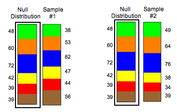
Of course, the distribution of color will vary in different samples, so we need to develop a way to measure how far a sample distribution is from the null distribution, something analogous to a z-score or T-score. Before we discuss this new measure, let’s look at two random samples selected from the null distribution to practice recognizing different amounts of variability. We can compare the distributions visually using ribbon charts.

Which random sample deviates the most from the null distribution? We address this question in the next activity.
Try It
Observed Counts for Two Random Samples
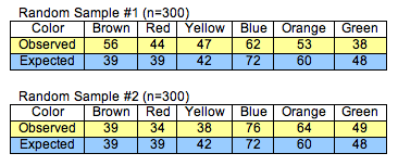
Here are the observed counts for the two random samples shown above. This is the same information shown in the ribbon charts.
Statisticians use the following formula to measure how far the observed data are from the null distribution. It is called the chi-square test statistic. The Greek letter chi is written χ.
Notes about this formula:
- Recall that the symbol ∑ means sum. Each category contributes a term to the sum, so the chi-square test statistic is based on the entire distribution. If the categorical variable has six categories, then the chi-square test statistic has six terms. If the categorical variable has three categories, then the chi-square test statistic has three terms, and so on.
- Notice that the difference “observed minus expected” for each category is part of the formula, but each difference is squared. This is necessary because the differences will add to 0, as we saw in the previous activity.
- Notice also that each squared difference is divided by the expected count for that category. The chi-square test statistic looks at the difference between the observed and expected counts relative to the size of the expected count.
Example
Calculating χ2
For Sample 1, the chi-square test statistic is approximately 12.94. For Sample 2, the chi-square test statistic is approximately 1.53. Usually, we use technology to calculate χ2, but here we show two calculations in detail to illustrate how the formula works. Notice that we are adding six terms. Each term represents the deviation for one color category.

Comment: In Sample 1, notice that both blue and green observed counts deviate from the expected counts by 10 candies. But green contributes more to the chi-square test statistic. This makes sense because the chi-square test statistic measures relative difference. Relative to the expected count of 48 green candies, an absolute error of 10 is large. It is almost 20% of the expected count. (10/48 is about 0.20). The squared difference relative to the expected count is 100/48, about 2.08. Relative to the expected count of 72 blue candies, an error of 10 candies is smaller. It is only about 14% of the expected count (10/72 is about 0.14). The squared difference relative to the expected count is 100/72, about 1.39.
Here is the chi-square calculation for Sample 2.

Calculating χ2
Contributors and Attributions
- Concepts in Statistics. Provided by: Open Learning Initiative. Located at: http://oli.cmu.edu. License: CC BY: Attribution


