10.19: Estimating a Population Mean (2 of 3)
- Page ID
- 14186
\( \newcommand{\vecs}[1]{\overset { \scriptstyle \rightharpoonup} {\mathbf{#1}} } \)
\( \newcommand{\vecd}[1]{\overset{-\!-\!\rightharpoonup}{\vphantom{a}\smash {#1}}} \)
\( \newcommand{\id}{\mathrm{id}}\) \( \newcommand{\Span}{\mathrm{span}}\)
( \newcommand{\kernel}{\mathrm{null}\,}\) \( \newcommand{\range}{\mathrm{range}\,}\)
\( \newcommand{\RealPart}{\mathrm{Re}}\) \( \newcommand{\ImaginaryPart}{\mathrm{Im}}\)
\( \newcommand{\Argument}{\mathrm{Arg}}\) \( \newcommand{\norm}[1]{\| #1 \|}\)
\( \newcommand{\inner}[2]{\langle #1, #2 \rangle}\)
\( \newcommand{\Span}{\mathrm{span}}\)
\( \newcommand{\id}{\mathrm{id}}\)
\( \newcommand{\Span}{\mathrm{span}}\)
\( \newcommand{\kernel}{\mathrm{null}\,}\)
\( \newcommand{\range}{\mathrm{range}\,}\)
\( \newcommand{\RealPart}{\mathrm{Re}}\)
\( \newcommand{\ImaginaryPart}{\mathrm{Im}}\)
\( \newcommand{\Argument}{\mathrm{Arg}}\)
\( \newcommand{\norm}[1]{\| #1 \|}\)
\( \newcommand{\inner}[2]{\langle #1, #2 \rangle}\)
\( \newcommand{\Span}{\mathrm{span}}\) \( \newcommand{\AA}{\unicode[.8,0]{x212B}}\)
\( \newcommand{\vectorA}[1]{\vec{#1}} % arrow\)
\( \newcommand{\vectorAt}[1]{\vec{\text{#1}}} % arrow\)
\( \newcommand{\vectorB}[1]{\overset { \scriptstyle \rightharpoonup} {\mathbf{#1}} } \)
\( \newcommand{\vectorC}[1]{\textbf{#1}} \)
\( \newcommand{\vectorD}[1]{\overrightarrow{#1}} \)
\( \newcommand{\vectorDt}[1]{\overrightarrow{\text{#1}}} \)
\( \newcommand{\vectE}[1]{\overset{-\!-\!\rightharpoonup}{\vphantom{a}\smash{\mathbf {#1}}}} \)
\( \newcommand{\vecs}[1]{\overset { \scriptstyle \rightharpoonup} {\mathbf{#1}} } \)
\( \newcommand{\vecd}[1]{\overset{-\!-\!\rightharpoonup}{\vphantom{a}\smash {#1}}} \)
\(\newcommand{\avec}{\mathbf a}\) \(\newcommand{\bvec}{\mathbf b}\) \(\newcommand{\cvec}{\mathbf c}\) \(\newcommand{\dvec}{\mathbf d}\) \(\newcommand{\dtil}{\widetilde{\mathbf d}}\) \(\newcommand{\evec}{\mathbf e}\) \(\newcommand{\fvec}{\mathbf f}\) \(\newcommand{\nvec}{\mathbf n}\) \(\newcommand{\pvec}{\mathbf p}\) \(\newcommand{\qvec}{\mathbf q}\) \(\newcommand{\svec}{\mathbf s}\) \(\newcommand{\tvec}{\mathbf t}\) \(\newcommand{\uvec}{\mathbf u}\) \(\newcommand{\vvec}{\mathbf v}\) \(\newcommand{\wvec}{\mathbf w}\) \(\newcommand{\xvec}{\mathbf x}\) \(\newcommand{\yvec}{\mathbf y}\) \(\newcommand{\zvec}{\mathbf z}\) \(\newcommand{\rvec}{\mathbf r}\) \(\newcommand{\mvec}{\mathbf m}\) \(\newcommand{\zerovec}{\mathbf 0}\) \(\newcommand{\onevec}{\mathbf 1}\) \(\newcommand{\real}{\mathbb R}\) \(\newcommand{\twovec}[2]{\left[\begin{array}{r}#1 \\ #2 \end{array}\right]}\) \(\newcommand{\ctwovec}[2]{\left[\begin{array}{c}#1 \\ #2 \end{array}\right]}\) \(\newcommand{\threevec}[3]{\left[\begin{array}{r}#1 \\ #2 \\ #3 \end{array}\right]}\) \(\newcommand{\cthreevec}[3]{\left[\begin{array}{c}#1 \\ #2 \\ #3 \end{array}\right]}\) \(\newcommand{\fourvec}[4]{\left[\begin{array}{r}#1 \\ #2 \\ #3 \\ #4 \end{array}\right]}\) \(\newcommand{\cfourvec}[4]{\left[\begin{array}{c}#1 \\ #2 \\ #3 \\ #4 \end{array}\right]}\) \(\newcommand{\fivevec}[5]{\left[\begin{array}{r}#1 \\ #2 \\ #3 \\ #4 \\ #5 \\ \end{array}\right]}\) \(\newcommand{\cfivevec}[5]{\left[\begin{array}{c}#1 \\ #2 \\ #3 \\ #4 \\ #5 \\ \end{array}\right]}\) \(\newcommand{\mattwo}[4]{\left[\begin{array}{rr}#1 \amp #2 \\ #3 \amp #4 \\ \end{array}\right]}\) \(\newcommand{\laspan}[1]{\text{Span}\{#1\}}\) \(\newcommand{\bcal}{\cal B}\) \(\newcommand{\ccal}{\cal C}\) \(\newcommand{\scal}{\cal S}\) \(\newcommand{\wcal}{\cal W}\) \(\newcommand{\ecal}{\cal E}\) \(\newcommand{\coords}[2]{\left\{#1\right\}_{#2}}\) \(\newcommand{\gray}[1]{\color{gray}{#1}}\) \(\newcommand{\lgray}[1]{\color{lightgray}{#1}}\) \(\newcommand{\rank}{\operatorname{rank}}\) \(\newcommand{\row}{\text{Row}}\) \(\newcommand{\col}{\text{Col}}\) \(\renewcommand{\row}{\text{Row}}\) \(\newcommand{\nul}{\text{Nul}}\) \(\newcommand{\var}{\text{Var}}\) \(\newcommand{\corr}{\text{corr}}\) \(\newcommand{\len}[1]{\left|#1\right|}\) \(\newcommand{\bbar}{\overline{\bvec}}\) \(\newcommand{\bhat}{\widehat{\bvec}}\) \(\newcommand{\bperp}{\bvec^\perp}\) \(\newcommand{\xhat}{\widehat{\xvec}}\) \(\newcommand{\vhat}{\widehat{\vvec}}\) \(\newcommand{\uhat}{\widehat{\uvec}}\) \(\newcommand{\what}{\widehat{\wvec}}\) \(\newcommand{\Sighat}{\widehat{\Sigma}}\) \(\newcommand{\lt}{<}\) \(\newcommand{\gt}{>}\) \(\newcommand{\amp}{&}\) \(\definecolor{fillinmathshade}{gray}{0.9}\)Learning Objectives
- Construct a confidence interval to estimate a population mean when conditions are met. Interpret the confidence interval in context.
- Interpret the meaning of a confidence level associated with a confidence interval.
- Adjust the margin of error by making changes to the confidence level or sample size.
On the previous page, we used a confidence interval to estimate the population mean, µ. For this confidence interval, we had to supply a guess for the population standard deviation, σ, based on previous studies. It may have occurred to you that if we do not know µ, it is unlikely that we know σ. So we now take a different approach. We estimate σ using the sample standard deviation, s.
This is the same type of adjustment we used in Inference for One Proportion when we had to adjust our model of the sampling distribution. The standard error of the sampling distribution is . (If we knew
, then we wouldn’t need to build a confidence interval.) We approximate
by the sample proportion,
.
Our process for adjusting the confidence interval for estimating µ is similar. We use the sample standard deviation, s, to estimate σ. The standard error for the sampling distribution becomes
. So we adjust the margin of error in the confidence interval formula, but this adjustment is not as straightforward as our work with proportions.
This estimate for σ introduces more uncertainty in the process. The problem is worse with smaller samples because the sample standard deviations vary more. For small samples, s is a worse approximation for σ. Unfortunately, this approximation makes the normal model a bad fit and inappropriate for determining critical values. We instead use what is called a t-model for this purpose.
Introduction to the T-Model
Here is the formula for the T-score. We also include the z-score for comparison. The formulas are very similar.
The distribution of z-scores is the standard normal curve, with mean of 0 and standard deviation of 1. The distribution of T-scores depends on the sample size, n. There is a different T-model for every n. So the T-model is a family of curves.
Instead of referring to n to specify which T-model to use, we refer to the degrees of freedom, or df for short. For Topics 10.2 and 10.3, the number of degrees of freedom is 1 less than the sample size. That is, df = n – 1.
In summary, a normal model is defined by its mean and standard deviation. A T-model is a family of curves defined by the degrees of freedom.
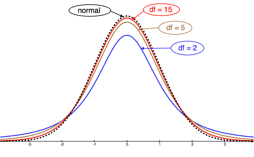
Let’s take a look at a few T-model curves (for various df) to see how they compare to the normal model.

We can see from the picture that as df grows, the T-model gets closer to the standard normal model.
Similarities between T-model and standard normal model:
- Symmetric with a central peak, bell-shaped.
- Centered at 0.
- The larger the degrees of freedom, the closer the T-model is to the standard normal model.
Difference between T-model and standard normal model:
- The T-model has more spread than the standard normal model.
- The T-model has more probability in the tails and less in the center than the standard normal model. We can see this in the fatter tails and lower central peak of the T-model.
When is a T-model a good fit for the sampling distribution of sample means?
Check these conditions before using the T-model:
- Use the T-model if σ (the population standard deviation) is unknown. If σ is known, then use the normal model instead of the T-model.
- Use the T-model if variable values are normally distributed in the population. If this is not true, then make sure the sample size is large (more than 30).
Example
Cable Strength
A group of engineers developed a new design for a steel cable. They need to estimate the amount of weight the cable can hold. The weight limit will be reported on cable packaging.
The engineers take a random sample of 45 cables and apply weights to each of them until they break. The mean breaking weight for the 45 cables is = 768.2 lb. The standard deviation of the breaking weight for the sample is s = 15.1 lb.
What should the engineers report as the mean amount of weight held by this type of cable?
Let’s use these sample statistics to construct a 95% confidence interval for the mean breaking weight of this type of cable.
Checking conditions:
Since we do not know the standard deviation of breaking weights of all of the cables (the population parameter σ), we use the sample standard deviation (s) as an approximation for σ. Since we don’t know σ, we must use the T-distribution to model the sampling distribution of means.
Is the T-model a good fit for the sampling distribution?
Yes, because the conditions are met:
- σ is unknown.
- The sample size is large enough.
Finding the standard error:
As usual, we start by estimating the standard error. This estimate comes from the formula . However, since we don’t know σ, we use s = 15.1 as an approximation for σ. So our estimate for the standard error of all sample means is
.
Finding the margin of error:
To find the margin of error, we need to find the critical T-value that corresponds to a 95% confidence level. This is just like the critical Z-value when we built confidence intervals for proportions, except that it comes from the T-model instead of the standard normal model.
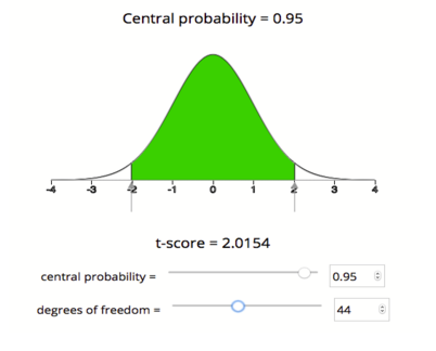
We will use technology to find the critical T-value. There are a number of tools for doing this. Some books will also give you the option to use printed tables of values. Here we will use a simulation that gives the T-model based on degrees of freedom. We want the T-values that cut off the central 95% of the area under the curve. It will look as follows.

Using the simulation, we see that the critical T-value for a 95% confidence interval with 44 degrees of freedom is Tc = 2.015, which means our margin of error for this confidence interval is
Note: For 95% confidence, the empirical rule approximates the critical Z-value as 2. The empirical rule is based on the normal model. Using the T-model for df = 44, the critical T-value (2.015) is very close to 2. This makes sense because for larger df, the T-model is very close to the standard normal model. We will see that the critical T-value differs more from the critical Z-value when the sample sizes are small.
Finding the confidence interval:
We have all the pieces to build the confidence interval. In our example, the confidence interval is
Conclusion:
We are 95% confident that the mean breaking weight for all cables of this type is between 763.7 lb and 772.7 lb.
Confidence intervals at the 95% confidence level are common in practice. But 95% is not the only confidence level we use. Particularly in situations that involve safety issues, such as the previous example, people often prefer to estimate population means with 99% confidence intervals. Let’s do some exploration with technology to see how changes in the confidence level affect the confidence interval.
Click here to open this simulation in its own window.
Try It
How Much Alcohol Do College Students Drink?
According to the website www.collegedrinkingprevention.gov, “About 25 percent of college students report academic consequences of their drinking including missing class, falling behind, doing poorly on exams or papers, and receiving lower grades overall.” A statistics student is curious about drinking habits of students at his college. He wants to estimate the mean number of alcoholic drinks consumed each week by students at his college. He plans to use a 90% confidence interval. He surveys a random sample of 71 students. The sample mean is 3.93 alcoholic drinks per week. The sample standard deviation is 3.78 drinks.
https://assessments.lumenlearning.co...sessments/3684
https://assessments.lumenlearning.co...sessments/3753
https://assessments.lumenlearning.co...sessments/3685
Contributors and Attributions
- Concepts in Statistics. Provided by: Open Learning Initiative. Located at: http://oli.cmu.edu. License: CC BY: Attribution

