
10.3: Estimating the Difference in Two Population Means
- Page ID
- 14170

\( \newcommand{\vecs}[1]{\overset { \scriptstyle \rightharpoonup} {\mathbf{#1}} } \)
\( \newcommand{\vecd}[1]{\overset{-\!-\!\rightharpoonup}{\vphantom{a}\smash {#1}}} \)
\( \newcommand{\dsum}{\displaystyle\sum\limits} \)
\( \newcommand{\dint}{\displaystyle\int\limits} \)
\( \newcommand{\dlim}{\displaystyle\lim\limits} \)
\( \newcommand{\id}{\mathrm{id}}\) \( \newcommand{\Span}{\mathrm{span}}\)
( \newcommand{\kernel}{\mathrm{null}\,}\) \( \newcommand{\range}{\mathrm{range}\,}\)
\( \newcommand{\RealPart}{\mathrm{Re}}\) \( \newcommand{\ImaginaryPart}{\mathrm{Im}}\)
\( \newcommand{\Argument}{\mathrm{Arg}}\) \( \newcommand{\norm}[1]{\| #1 \|}\)
\( \newcommand{\inner}[2]{\langle #1, #2 \rangle}\)
\( \newcommand{\Span}{\mathrm{span}}\)
\( \newcommand{\id}{\mathrm{id}}\)
\( \newcommand{\Span}{\mathrm{span}}\)
\( \newcommand{\kernel}{\mathrm{null}\,}\)
\( \newcommand{\range}{\mathrm{range}\,}\)
\( \newcommand{\RealPart}{\mathrm{Re}}\)
\( \newcommand{\ImaginaryPart}{\mathrm{Im}}\)
\( \newcommand{\Argument}{\mathrm{Arg}}\)
\( \newcommand{\norm}[1]{\| #1 \|}\)
\( \newcommand{\inner}[2]{\langle #1, #2 \rangle}\)
\( \newcommand{\Span}{\mathrm{span}}\) \( \newcommand{\AA}{\unicode[.8,0]{x212B}}\)
\( \newcommand{\vectorA}[1]{\vec{#1}} % arrow\)
\( \newcommand{\vectorAt}[1]{\vec{\text{#1}}} % arrow\)
\( \newcommand{\vectorB}[1]{\overset { \scriptstyle \rightharpoonup} {\mathbf{#1}} } \)
\( \newcommand{\vectorC}[1]{\textbf{#1}} \)
\( \newcommand{\vectorD}[1]{\overrightarrow{#1}} \)
\( \newcommand{\vectorDt}[1]{\overrightarrow{\text{#1}}} \)
\( \newcommand{\vectE}[1]{\overset{-\!-\!\rightharpoonup}{\vphantom{a}\smash{\mathbf {#1}}}} \)
\( \newcommand{\vecs}[1]{\overset { \scriptstyle \rightharpoonup} {\mathbf{#1}} } \)
\(\newcommand{\longvect}{\overrightarrow}\)
\( \newcommand{\vecd}[1]{\overset{-\!-\!\rightharpoonup}{\vphantom{a}\smash {#1}}} \)
\(\newcommand{\avec}{\mathbf a}\) \(\newcommand{\bvec}{\mathbf b}\) \(\newcommand{\cvec}{\mathbf c}\) \(\newcommand{\dvec}{\mathbf d}\) \(\newcommand{\dtil}{\widetilde{\mathbf d}}\) \(\newcommand{\evec}{\mathbf e}\) \(\newcommand{\fvec}{\mathbf f}\) \(\newcommand{\nvec}{\mathbf n}\) \(\newcommand{\pvec}{\mathbf p}\) \(\newcommand{\qvec}{\mathbf q}\) \(\newcommand{\svec}{\mathbf s}\) \(\newcommand{\tvec}{\mathbf t}\) \(\newcommand{\uvec}{\mathbf u}\) \(\newcommand{\vvec}{\mathbf v}\) \(\newcommand{\wvec}{\mathbf w}\) \(\newcommand{\xvec}{\mathbf x}\) \(\newcommand{\yvec}{\mathbf y}\) \(\newcommand{\zvec}{\mathbf z}\) \(\newcommand{\rvec}{\mathbf r}\) \(\newcommand{\mvec}{\mathbf m}\) \(\newcommand{\zerovec}{\mathbf 0}\) \(\newcommand{\onevec}{\mathbf 1}\) \(\newcommand{\real}{\mathbb R}\) \(\newcommand{\twovec}[2]{\left[\begin{array}{r}#1 \\ #2 \end{array}\right]}\) \(\newcommand{\ctwovec}[2]{\left[\begin{array}{c}#1 \\ #2 \end{array}\right]}\) \(\newcommand{\threevec}[3]{\left[\begin{array}{r}#1 \\ #2 \\ #3 \end{array}\right]}\) \(\newcommand{\cthreevec}[3]{\left[\begin{array}{c}#1 \\ #2 \\ #3 \end{array}\right]}\) \(\newcommand{\fourvec}[4]{\left[\begin{array}{r}#1 \\ #2 \\ #3 \\ #4 \end{array}\right]}\) \(\newcommand{\cfourvec}[4]{\left[\begin{array}{c}#1 \\ #2 \\ #3 \\ #4 \end{array}\right]}\) \(\newcommand{\fivevec}[5]{\left[\begin{array}{r}#1 \\ #2 \\ #3 \\ #4 \\ #5 \\ \end{array}\right]}\) \(\newcommand{\cfivevec}[5]{\left[\begin{array}{c}#1 \\ #2 \\ #3 \\ #4 \\ #5 \\ \end{array}\right]}\) \(\newcommand{\mattwo}[4]{\left[\begin{array}{rr}#1 \amp #2 \\ #3 \amp #4 \\ \end{array}\right]}\) \(\newcommand{\laspan}[1]{\text{Span}\{#1\}}\) \(\newcommand{\bcal}{\cal B}\) \(\newcommand{\ccal}{\cal C}\) \(\newcommand{\scal}{\cal S}\) \(\newcommand{\wcal}{\cal W}\) \(\newcommand{\ecal}{\cal E}\) \(\newcommand{\coords}[2]{\left\{#1\right\}_{#2}}\) \(\newcommand{\gray}[1]{\color{gray}{#1}}\) \(\newcommand{\lgray}[1]{\color{lightgray}{#1}}\) \(\newcommand{\rank}{\operatorname{rank}}\) \(\newcommand{\row}{\text{Row}}\) \(\newcommand{\col}{\text{Col}}\) \(\renewcommand{\row}{\text{Row}}\) \(\newcommand{\nul}{\text{Nul}}\) \(\newcommand{\var}{\text{Var}}\) \(\newcommand{\corr}{\text{corr}}\) \(\newcommand{\len}[1]{\left|#1\right|}\) \(\newcommand{\bbar}{\overline{\bvec}}\) \(\newcommand{\bhat}{\widehat{\bvec}}\) \(\newcommand{\bperp}{\bvec^\perp}\) \(\newcommand{\xhat}{\widehat{\xvec}}\) \(\newcommand{\vhat}{\widehat{\vvec}}\) \(\newcommand{\uhat}{\widehat{\uvec}}\) \(\newcommand{\what}{\widehat{\wvec}}\) \(\newcommand{\Sighat}{\widehat{\Sigma}}\) \(\newcommand{\lt}{<}\) \(\newcommand{\gt}{>}\) \(\newcommand{\amp}{&}\) \(\definecolor{fillinmathshade}{gray}{0.9}\)Learning Objectives
- Construct a confidence interval to estimate a difference in two population means (when conditions are met). Interpret the confidence interval in context.
Confidence Interval to Estimate μ1 − μ2
In a hypothesis test, when the sample evidence leads us to reject the null hypothesis, we conclude that the population means differ or that one is larger than the other. An obvious next question is how much larger? In practice, when the sample mean difference is statistically significant, our next step is often to calculate a confidence interval to estimate the size of the population mean difference.
The confidence interval gives us a range of reasonable values for the difference in population means μ1 − μ2. We call this the two-sample T-interval or the confidence interval to estimate a difference in two population means. The form of the confidence interval is similar to others we have seen.
Sample Statistic
Since we’re estimating the difference between two population means, the sample statistic is the difference between the means of the two independent samples: .
Critical T-Value
The critical T-value comes from the T-model, just as it did in “Estimating a Population Mean.” Again, this value depends on the degrees of freedom (df). For two-sample T-test or two-sample T-intervals, the df value is based on a complicated formula that we do not cover in this course. We either give the df or use technology to find the df.
Standard Error
The estimated standard error for the two-sample T-interval is the same formula we used for the two-sample T-test. (As usual, s1 and s2 denote the sample standard deviations, and n1 and n2 denote the sample sizes.)
Putting all this together gives us the following formula for the two-sample T-interval.
Conditions for Use
The conditions for using this two-sample T-interval are the same as the conditions for using the two-sample T-test.
- The two random samples are independent and representative.
- The variable is normally distributed in both populations. If it is not known, samples of more than 30 will have a difference in sample means that can be modeled adequately by the T-distribution. As we discussed in “Hypothesis Test for a Population Mean,” T-procedures are robust even when the variable is not normally distributed in the population. If checking normality in the populations is impossible, then we look at the distribution in the samples. If a histogram or dotplot of the data does not show extreme skew or outliers, we take it as a sign that the variable is not heavily skewed in the populations, and we use the inference procedure.
Example
Confidence Interval for the “Calories and Context” Study
In the preceding few pages, we worked through a two-sample T-test for the “calories and context” example. In this example, we use the sample data to find a two-sample T-interval for μ1 − μ2 at the 95% confidence level.
Recap of the Situation
- Population 1: Let μ1 be the mean number of calories purchased by women eating with other women.
- Population 2: Let μ2 be the mean number of calories purchased by women eating with men.
Sample Statistics
| Size (n) | SD (s) | ||
|---|---|---|---|
| Sample 1 | 45 | 850 | 252 |
| Sample 2 | 27 | 719 | 322 |
Standard Error
We found that the standard error of the sampling distribution of all sample differences is approximately 72.47.
Critical T-value
For these two independent samples, df = 45. We find the critical T-value using the same simulation we used in “Estimating a Population Mean.”
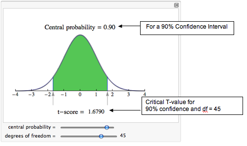
Reading from the simulation, we see that the critical T-value is 1.6790.
Confidence Interval
We can now put all this together to compute the confidence interval:
Expressing this as an interval gives us:
Interpretation
We are 95% confident that the true value of μ1 − μ2 is between 9 and 253 calories. We can be more specific about the populations. We are 95% confident that at Indiana University of Pennsylvania, undergraduate women eating with women order between 9.32 and 252.68 more calories than undergraduate women eating with men.
In this next activity, we focus on interpreting confidence intervals and evaluating a statistics project conducted by students in an introductory statistics course.
Try It
Improving Children’s Math Skills
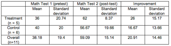
Students in an introductory statistics course at Los Medanos College designed an experiment to study the impact of subliminal messages on improving children’s math skills. The students were inspired by a similar study at City University of New York, as described in David Moore’s textbook The Basic Practice of Statistics(4th ed., W. H. Freeman, 2007). The participants were 11 children who attended an afterschool tutoring program at a local church. The children ranged in age from 8 to 11. All received tutoring in arithmetic skills. At the beginning of each tutoring session, the children watched a short video with a religious message that ended with a promotional message for the church.
The statistics students added a slide that said, “I work hard and I am good at math.” This slide flashed quickly during the promotional message, so quickly that no one was aware of the slide. Children who attended the tutoring sessions on Mondays watched the video with the extra slide. Children who attended the tutoring sessions on Wednesday watched the video without the extra slide. The experiment lasted 4 weeks. The children took a pretest and posttest in arithmetic. Here are some of the results:
 https://assessments.lumenlearning.co...sessments/3714
Let’s Summarize
Hypothesis tests and confidence intervals for two means can answer research questions about two populations or two treatments that involve quantitative data. In “Inference for a Difference between Population Means,” we focused on studies that produced two independent samples. Previously, in “Hpyothesis Test for a Population Mean,” we looked at matched-pairs studies in which individual data points in one sample are naturally paired with the individual data points in the other sample.
The hypotheses for two population means are similar to those for two population proportions.
The null hypothesis, H0, is a statement of “no effect” or “no difference.”
- H0: μ1 – μ2 = 0, which is the same as H0: μ1 = μ2
The alternative hypothesis, Ha, takes one of the following three forms:
- Ha: μ1 – μ2 < 0, which is the same as Ha: μ1 < μ2
- Ha: μ1 – μ2 > 0, which is the same as Ha: μ1 > μ2
- Ha: μ1 – μ2 ≠ 0, which is the same as Ha: μ1 ≠ μ2
As usual, how we collect the data determines whether we can use it in the inference procedure. We have our usual two requirements for data collection.
- Samples must be random in order to remove or minimize bias.
- Sample must be representative of the population in question.
We use the two-sample hypothesis test and confidence interval when the following conditions are met:
- The two random samples are independent.
- The variable is normally distributed in both populations. If this variable is not known, samples of more than 30 will have a difference in sample means that can be modeled adequately by the t-distribution. As we discussed in “Hypothesis Test for a Population Mean,” t-procedures are robust even when the variable is not normally distributed in the population. Therefore, if checking normality in the populations is impossible, then we look at the distribution in the samples. If a histogram or dotplot of the data does not show extreme skew or outliers, we take it as a sign that the variable is not heavily skewed in the populations, and we use the inference procedure.
Formulas:
The confidence interval for μ1 − μ2 is
Hypothesis test for H0: μ1 – μ2 = 0 is
We use technology to find the degrees of freedom to determine P-values and critical t-values for confidence intervals. (In most problems in this section, we provided the degrees of freedom for you.)
Contributors and Attributions
- Concepts in Statistics. Provided by: Open Learning Initiative. Located at: http://oli.cmu.edu. License: CC BY: Attribution