7.5: Distribution of Sample Proportions (2 of 6)
- Page ID
- 14115
\( \newcommand{\vecs}[1]{\overset { \scriptstyle \rightharpoonup} {\mathbf{#1}} } \)
\( \newcommand{\vecd}[1]{\overset{-\!-\!\rightharpoonup}{\vphantom{a}\smash {#1}}} \)
\( \newcommand{\id}{\mathrm{id}}\) \( \newcommand{\Span}{\mathrm{span}}\)
( \newcommand{\kernel}{\mathrm{null}\,}\) \( \newcommand{\range}{\mathrm{range}\,}\)
\( \newcommand{\RealPart}{\mathrm{Re}}\) \( \newcommand{\ImaginaryPart}{\mathrm{Im}}\)
\( \newcommand{\Argument}{\mathrm{Arg}}\) \( \newcommand{\norm}[1]{\| #1 \|}\)
\( \newcommand{\inner}[2]{\langle #1, #2 \rangle}\)
\( \newcommand{\Span}{\mathrm{span}}\)
\( \newcommand{\id}{\mathrm{id}}\)
\( \newcommand{\Span}{\mathrm{span}}\)
\( \newcommand{\kernel}{\mathrm{null}\,}\)
\( \newcommand{\range}{\mathrm{range}\,}\)
\( \newcommand{\RealPart}{\mathrm{Re}}\)
\( \newcommand{\ImaginaryPart}{\mathrm{Im}}\)
\( \newcommand{\Argument}{\mathrm{Arg}}\)
\( \newcommand{\norm}[1]{\| #1 \|}\)
\( \newcommand{\inner}[2]{\langle #1, #2 \rangle}\)
\( \newcommand{\Span}{\mathrm{span}}\) \( \newcommand{\AA}{\unicode[.8,0]{x212B}}\)
\( \newcommand{\vectorA}[1]{\vec{#1}} % arrow\)
\( \newcommand{\vectorAt}[1]{\vec{\text{#1}}} % arrow\)
\( \newcommand{\vectorB}[1]{\overset { \scriptstyle \rightharpoonup} {\mathbf{#1}} } \)
\( \newcommand{\vectorC}[1]{\textbf{#1}} \)
\( \newcommand{\vectorD}[1]{\overrightarrow{#1}} \)
\( \newcommand{\vectorDt}[1]{\overrightarrow{\text{#1}}} \)
\( \newcommand{\vectE}[1]{\overset{-\!-\!\rightharpoonup}{\vphantom{a}\smash{\mathbf {#1}}}} \)
\( \newcommand{\vecs}[1]{\overset { \scriptstyle \rightharpoonup} {\mathbf{#1}} } \)
\( \newcommand{\vecd}[1]{\overset{-\!-\!\rightharpoonup}{\vphantom{a}\smash {#1}}} \)
\(\newcommand{\avec}{\mathbf a}\) \(\newcommand{\bvec}{\mathbf b}\) \(\newcommand{\cvec}{\mathbf c}\) \(\newcommand{\dvec}{\mathbf d}\) \(\newcommand{\dtil}{\widetilde{\mathbf d}}\) \(\newcommand{\evec}{\mathbf e}\) \(\newcommand{\fvec}{\mathbf f}\) \(\newcommand{\nvec}{\mathbf n}\) \(\newcommand{\pvec}{\mathbf p}\) \(\newcommand{\qvec}{\mathbf q}\) \(\newcommand{\svec}{\mathbf s}\) \(\newcommand{\tvec}{\mathbf t}\) \(\newcommand{\uvec}{\mathbf u}\) \(\newcommand{\vvec}{\mathbf v}\) \(\newcommand{\wvec}{\mathbf w}\) \(\newcommand{\xvec}{\mathbf x}\) \(\newcommand{\yvec}{\mathbf y}\) \(\newcommand{\zvec}{\mathbf z}\) \(\newcommand{\rvec}{\mathbf r}\) \(\newcommand{\mvec}{\mathbf m}\) \(\newcommand{\zerovec}{\mathbf 0}\) \(\newcommand{\onevec}{\mathbf 1}\) \(\newcommand{\real}{\mathbb R}\) \(\newcommand{\twovec}[2]{\left[\begin{array}{r}#1 \\ #2 \end{array}\right]}\) \(\newcommand{\ctwovec}[2]{\left[\begin{array}{c}#1 \\ #2 \end{array}\right]}\) \(\newcommand{\threevec}[3]{\left[\begin{array}{r}#1 \\ #2 \\ #3 \end{array}\right]}\) \(\newcommand{\cthreevec}[3]{\left[\begin{array}{c}#1 \\ #2 \\ #3 \end{array}\right]}\) \(\newcommand{\fourvec}[4]{\left[\begin{array}{r}#1 \\ #2 \\ #3 \\ #4 \end{array}\right]}\) \(\newcommand{\cfourvec}[4]{\left[\begin{array}{c}#1 \\ #2 \\ #3 \\ #4 \end{array}\right]}\) \(\newcommand{\fivevec}[5]{\left[\begin{array}{r}#1 \\ #2 \\ #3 \\ #4 \\ #5 \\ \end{array}\right]}\) \(\newcommand{\cfivevec}[5]{\left[\begin{array}{c}#1 \\ #2 \\ #3 \\ #4 \\ #5 \\ \end{array}\right]}\) \(\newcommand{\mattwo}[4]{\left[\begin{array}{rr}#1 \amp #2 \\ #3 \amp #4 \\ \end{array}\right]}\) \(\newcommand{\laspan}[1]{\text{Span}\{#1\}}\) \(\newcommand{\bcal}{\cal B}\) \(\newcommand{\ccal}{\cal C}\) \(\newcommand{\scal}{\cal S}\) \(\newcommand{\wcal}{\cal W}\) \(\newcommand{\ecal}{\cal E}\) \(\newcommand{\coords}[2]{\left\{#1\right\}_{#2}}\) \(\newcommand{\gray}[1]{\color{gray}{#1}}\) \(\newcommand{\lgray}[1]{\color{lightgray}{#1}}\) \(\newcommand{\rank}{\operatorname{rank}}\) \(\newcommand{\row}{\text{Row}}\) \(\newcommand{\col}{\text{Col}}\) \(\renewcommand{\row}{\text{Row}}\) \(\newcommand{\nul}{\text{Nul}}\) \(\newcommand{\var}{\text{Var}}\) \(\newcommand{\corr}{\text{corr}}\) \(\newcommand{\len}[1]{\left|#1\right|}\) \(\newcommand{\bbar}{\overline{\bvec}}\) \(\newcommand{\bhat}{\widehat{\bvec}}\) \(\newcommand{\bperp}{\bvec^\perp}\) \(\newcommand{\xhat}{\widehat{\xvec}}\) \(\newcommand{\vhat}{\widehat{\vvec}}\) \(\newcommand{\uhat}{\widehat{\uvec}}\) \(\newcommand{\what}{\widehat{\wvec}}\) \(\newcommand{\Sighat}{\widehat{\Sigma}}\) \(\newcommand{\lt}{<}\) \(\newcommand{\gt}{>}\) \(\newcommand{\amp}{&}\) \(\definecolor{fillinmathshade}{gray}{0.9}\)Learning Objectives
- Describe the sampling distribution for sample proportions and use it to identify unusual (and more common) sample results.
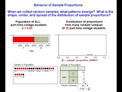
Recall that our goal is to create a probability model that describes the long-run behavior of proportions from random samples. Previously, we used a simulation to collect a few random samples to get acquainted with making a distribution of sample proportions. We randomly selected 25 students at a time from a population of part-time college students that is 60% female. In the next example, we predict what happens in the long run when we select many, many random samples of 25 students at a time from this population. Then we watch a simulation to see if our predictions are correct.
Example
Predicting the Behavior of Sample Proportions
Based on our intuition and what we observed with the simulation, we might expect the following about the distribution of sample proportions that come from a population where p = 0.60:
Center: Some sample proportions will be on the low side – such as 0.52 or 0.56 – and others will be on the high side – such as 0.64 or 0.68. It is reasonable to expect all the sample proportions in repeated random samples to average out to the underlying population proportion, 0.6. In other words, the mean of the distribution of sample proportions should be p.
Spread: For samples of 25, we expect sample proportions of females not to stray too far from the population proportion 0.6. Sample proportions lower than 0.44 or higher than 0.72 will be unusual. Previously, we took smaller random samples of 8 and observed more variability in the sample proportions. We therefore think that sample size plays a role in the spread of the distribution of sample proportions. Smaller samples may be less accurate and more variable than larger samples.
Shape: Sample proportions closest to 0.6 will be most common, and sample proportions far from 0.6 in either direction will be progressively less likely. In other words, the shape of the distribution of sample proportions may be somewhat bell-shaped.
Now we use a simulation to collect numerous samples to see what happens in the long run. We use the simulation to check whether our intuition about the center, spread, and shape of the distribution of sample proportions is right.
At this point, we have a good sense of what happens as we take random samples from a population. Our simulation suggests that our initial intuition about the shape and center of the distribution of sample proportions is correct.
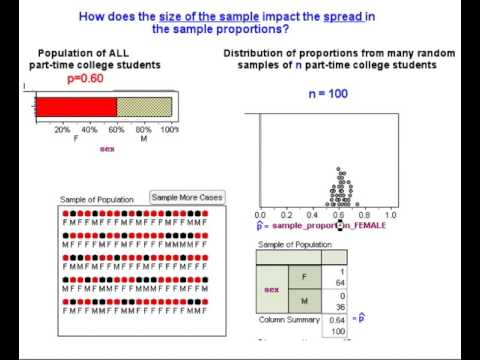
Now we use another simulation to help us think more precisely about the variability we expect to see in the sample proportions. Our intuition tells us that larger samples will better approximate the population, so we might expect less variability in large samples. In the next walk-through, we use a simulation to investigate this idea. After that walk-through, we tie these ideas to more formal theory about the probability model for the long-run behavior of proportions from random samples.
We are now ready to use what we have observed to develop a formal probability model to describe the behavior of sample proportions. First, let’s return to the original question that prompted our investigation of sample proportions.
We based our investigation on the prediction that 60% of part-time college students will be female. In our investigation, we asked, How much could the sample proportion vary from a population proportion of 0.60 for us to feel confident in our prediction?
We don’t expect a sample proportion to be exactly equal to the population proportion. But how much error seems reasonable?
We now see that the answer to this question depends on the size of the sample.
- If we select a random sample of 25 students, the distribution of sample proportions has a standard deviation of about 0.1. We can see that most sample proportions fall within 2 standard deviations of 0.60. Therefore, we might decide that 2 × 0.10 = 0.20 is a reasonable margin of error, so a sample proportion between 0.40 and 0.80 is not surprising if 0.60 of all part-time college students are female.
- If we select a random sample of 100 students, the distribution of sample proportions has less variability. It has a standard deviation of about 0.05. Again we see that most sample proportions fall within 2 standard deviations of 0.60, so we might decide that 2 × 0.05 = 0.10 is a reasonable amount of error for these larger samples. For a sample of 100 students, then, a sample proportion between 0.50 and 0.70 is not surprising if 0.60 of all part-time college students are female.
We discuss this idea further in “Introduction to Statistical Inference” in this unit.
Contributors and Attributions
- Concepts in Statistics. Provided by: Open Learning Initiative. Located at: http://oli.cmu.edu. License: CC BY: Attribution


