
6.6: Normal Random Variables (6 of 6)
- Page ID
- 14096
\( \newcommand{\vecs}[1]{\overset { \scriptstyle \rightharpoonup} {\mathbf{#1}} } \)
\( \newcommand{\vecd}[1]{\overset{-\!-\!\rightharpoonup}{\vphantom{a}\smash {#1}}} \)
\( \newcommand{\id}{\mathrm{id}}\) \( \newcommand{\Span}{\mathrm{span}}\)
( \newcommand{\kernel}{\mathrm{null}\,}\) \( \newcommand{\range}{\mathrm{range}\,}\)
\( \newcommand{\RealPart}{\mathrm{Re}}\) \( \newcommand{\ImaginaryPart}{\mathrm{Im}}\)
\( \newcommand{\Argument}{\mathrm{Arg}}\) \( \newcommand{\norm}[1]{\| #1 \|}\)
\( \newcommand{\inner}[2]{\langle #1, #2 \rangle}\)
\( \newcommand{\Span}{\mathrm{span}}\)
\( \newcommand{\id}{\mathrm{id}}\)
\( \newcommand{\Span}{\mathrm{span}}\)
\( \newcommand{\kernel}{\mathrm{null}\,}\)
\( \newcommand{\range}{\mathrm{range}\,}\)
\( \newcommand{\RealPart}{\mathrm{Re}}\)
\( \newcommand{\ImaginaryPart}{\mathrm{Im}}\)
\( \newcommand{\Argument}{\mathrm{Arg}}\)
\( \newcommand{\norm}[1]{\| #1 \|}\)
\( \newcommand{\inner}[2]{\langle #1, #2 \rangle}\)
\( \newcommand{\Span}{\mathrm{span}}\) \( \newcommand{\AA}{\unicode[.8,0]{x212B}}\)
\( \newcommand{\vectorA}[1]{\vec{#1}} % arrow\)
\( \newcommand{\vectorAt}[1]{\vec{\text{#1}}} % arrow\)
\( \newcommand{\vectorB}[1]{\overset { \scriptstyle \rightharpoonup} {\mathbf{#1}} } \)
\( \newcommand{\vectorC}[1]{\textbf{#1}} \)
\( \newcommand{\vectorD}[1]{\overrightarrow{#1}} \)
\( \newcommand{\vectorDt}[1]{\overrightarrow{\text{#1}}} \)
\( \newcommand{\vectE}[1]{\overset{-\!-\!\rightharpoonup}{\vphantom{a}\smash{\mathbf {#1}}}} \)
\( \newcommand{\vecs}[1]{\overset { \scriptstyle \rightharpoonup} {\mathbf{#1}} } \)
\( \newcommand{\vecd}[1]{\overset{-\!-\!\rightharpoonup}{\vphantom{a}\smash {#1}}} \)
\(\newcommand{\avec}{\mathbf a}\) \(\newcommand{\bvec}{\mathbf b}\) \(\newcommand{\cvec}{\mathbf c}\) \(\newcommand{\dvec}{\mathbf d}\) \(\newcommand{\dtil}{\widetilde{\mathbf d}}\) \(\newcommand{\evec}{\mathbf e}\) \(\newcommand{\fvec}{\mathbf f}\) \(\newcommand{\nvec}{\mathbf n}\) \(\newcommand{\pvec}{\mathbf p}\) \(\newcommand{\qvec}{\mathbf q}\) \(\newcommand{\svec}{\mathbf s}\) \(\newcommand{\tvec}{\mathbf t}\) \(\newcommand{\uvec}{\mathbf u}\) \(\newcommand{\vvec}{\mathbf v}\) \(\newcommand{\wvec}{\mathbf w}\) \(\newcommand{\xvec}{\mathbf x}\) \(\newcommand{\yvec}{\mathbf y}\) \(\newcommand{\zvec}{\mathbf z}\) \(\newcommand{\rvec}{\mathbf r}\) \(\newcommand{\mvec}{\mathbf m}\) \(\newcommand{\zerovec}{\mathbf 0}\) \(\newcommand{\onevec}{\mathbf 1}\) \(\newcommand{\real}{\mathbb R}\) \(\newcommand{\twovec}[2]{\left[\begin{array}{r}#1 \\ #2 \end{array}\right]}\) \(\newcommand{\ctwovec}[2]{\left[\begin{array}{c}#1 \\ #2 \end{array}\right]}\) \(\newcommand{\threevec}[3]{\left[\begin{array}{r}#1 \\ #2 \\ #3 \end{array}\right]}\) \(\newcommand{\cthreevec}[3]{\left[\begin{array}{c}#1 \\ #2 \\ #3 \end{array}\right]}\) \(\newcommand{\fourvec}[4]{\left[\begin{array}{r}#1 \\ #2 \\ #3 \\ #4 \end{array}\right]}\) \(\newcommand{\cfourvec}[4]{\left[\begin{array}{c}#1 \\ #2 \\ #3 \\ #4 \end{array}\right]}\) \(\newcommand{\fivevec}[5]{\left[\begin{array}{r}#1 \\ #2 \\ #3 \\ #4 \\ #5 \\ \end{array}\right]}\) \(\newcommand{\cfivevec}[5]{\left[\begin{array}{c}#1 \\ #2 \\ #3 \\ #4 \\ #5 \\ \end{array}\right]}\) \(\newcommand{\mattwo}[4]{\left[\begin{array}{rr}#1 \amp #2 \\ #3 \amp #4 \\ \end{array}\right]}\) \(\newcommand{\laspan}[1]{\text{Span}\{#1\}}\) \(\newcommand{\bcal}{\cal B}\) \(\newcommand{\ccal}{\cal C}\) \(\newcommand{\scal}{\cal S}\) \(\newcommand{\wcal}{\cal W}\) \(\newcommand{\ecal}{\cal E}\) \(\newcommand{\coords}[2]{\left\{#1\right\}_{#2}}\) \(\newcommand{\gray}[1]{\color{gray}{#1}}\) \(\newcommand{\lgray}[1]{\color{lightgray}{#1}}\) \(\newcommand{\rank}{\operatorname{rank}}\) \(\newcommand{\row}{\text{Row}}\) \(\newcommand{\col}{\text{Col}}\) \(\renewcommand{\row}{\text{Row}}\) \(\newcommand{\nul}{\text{Nul}}\) \(\newcommand{\var}{\text{Var}}\) \(\newcommand{\corr}{\text{corr}}\) \(\newcommand{\len}[1]{\left|#1\right|}\) \(\newcommand{\bbar}{\overline{\bvec}}\) \(\newcommand{\bhat}{\widehat{\bvec}}\) \(\newcommand{\bperp}{\bvec^\perp}\) \(\newcommand{\xhat}{\widehat{\xvec}}\) \(\newcommand{\vhat}{\widehat{\vvec}}\) \(\newcommand{\uhat}{\widehat{\uvec}}\) \(\newcommand{\what}{\widehat{\wvec}}\) \(\newcommand{\Sighat}{\widehat{\Sigma}}\) \(\newcommand{\lt}{<}\) \(\newcommand{\gt}{>}\) \(\newcommand{\amp}{&}\) \(\definecolor{fillinmathshade}{gray}{0.9}\)Learning Objectives
- Use a normal probability distribution to estimate probabilities and identify unusual events.
Now we use the simulation and the standard normal curve to find the probabilities associated with any normal density curve.
Example
Length of Human Pregnancy
The length (in days) of a randomly chosen human pregnancy is a normal random variable with μ = 266, σ = 16. So X = length of pregnancy (in days)
(a) What is the probability that a randomly chosen pregnancy will last less than 246 days?
We want P(X < 246). To find this probability, we first convert X = 246 to a z-score:
Now we can use the simulation to find P(Z < −1.25). This is the area under the normal probability curve to the left of Z = −1.25.

The probability that a randomly chosen pregnancy lasts less than 246 days is 0.1056. In other words, there is an 11% chance that a randomly selected pregnancy will last less than 246 days.
(b) Suppose a pregnant woman’s husband has scheduled his business trips so that he will be in town between the 235th and 295th days of her pregnancy. What is the probability that the birth will take place during that time?
Compute the z-scores for each of these x-values:
and
Use the simulation to find the area under the standard normal curve between these two z-scores.

So the desired probability is 0.9387.
There is about a 94% probability that he will be home for the birth. Looks like he planned well.
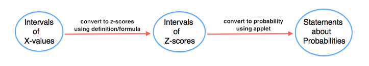
The previous examples all followed the same general form: Given values of a normal random variable, we found an associated probability. The two basic steps in the solution process were as follows:
- Convert x-value to a z-score.
- Use the simulation to find associated probability.
The next example is a different type of problem: Given a probability, we will find the associated value of the normal random variable. The solution process will go in reverse order.
- Use a new simulation to convert statements about probabilities to statements about z-scores.
- Convert z-scores to x-values.
These types of problems are informally called “work-backwards” problems. We will use a new simulation for these types of problems. The new simulation requires us to enter a probability and then gives us the associated z-score. This is backwards from the simulation we worked with previously where we entered a z-score to find a probability. We will use this simulation in the next example.
Click here to open this simulation in its own window.
Example
Work Backwards to Find X
Foot length (in inches) of a randomly chosen adult male is a normal random variable with a mean of 11 and standard deviation of 1.5. So X = foot length (inches).
(a) Suppose that an XL sock is designed to fit the largest 30% of men’s feet. What is the smallest foot length that fits an XL sock?
Step 1: Use the simulation to convert the probability to a statement about z-scores.
We want to mark off the largest 30% of the distribution, so the probability to the right of the z-score is 30%. This means that 70% of the area is to the left of the z-score.

From the simulation, we can see that the corresponding z-score is 0.52.
Step 2: Now we need to convert this z-score to a foot length.
Before we calculate the length, note that the z-score is about 0.5, so the x-value will be about 0.5 standard deviations above the mean.
Conclusion: A foot length of 11.75 inches is the shortest foot for an XL sock.
(b) What is the first quartile for the men’s foot lengths?
Step 1: Use the simulation to convert this probability into a statement about z-scores.
We want to mark off the smallest 25% of the distribution, so the probability to the left of the z-score is 25%.

From the simulation, we can see that the corresponding z-score is −0.67.
Step 2: Convert this z-score to a foot length. If X is the foot length we seek, then X is 0.67 standard deviations below the mean. That is,
Conclusion: The first quartile mark is 9.995 inches, so about 25% of the men’s feet are shorter than 10 inches.
Comments
In the preceding example (specifically step 2), we found the x-value by reasoning about the meaning of the z-score. We can also develop a formula for this process.
Recall the definition of z-score. In words, the z-score of an x-value is the number of standard deviations X is away from the mean. As a formula, this is
We can solve this equation for X as follows:
This gives us a formula for finding X from Z. You can use this formula in step 2 of a work-backwards problem.
Let’s Summarize
- In “Continuous Random Variables,” we made the transition from discrete to continuous random variables. A continuous random variable is not limited to distinct values. It is a measurement such as foot length. We cannot display the probability distribution for a continuous random variable with a table or histogram. We use a density curve to assign probabilities to intervals of x-values. We use the area under the density curve to find probabilities.
- We use a normal density curve to model the probability distribution for many variables, such as weight, shoe sizes, foot lengths, and other human physical characteristics. Normal curves are mathematical models. We use µ to represent the mean of a normal curve and σ to represent the standard deviation of a normal curve. We use Greek letters to remind us that the normal curve is not a distribution of real data. It is a mathematical model based on a mathematical equation. We use this mathematical model to represent the perfect bell-shaped distribution.
- For a normal curve, the empirical rule for normal curves tells us that 68% of the observations fall within 1 standard deviation of the mean, 95% within 2 standard deviations of the mean, and 99.7% within 3 standard deviations of the mean.
- To compare x-values from different distributions, we standardize the values by finding a z-score:
- A z-score measures how far X is from the mean in standard deviations. In other words, the z-score is the number of standard deviations X is from the mean of the distribution. For example, Z = 1 means the x-value is 1 standard deviation above the mean.
- If we convert the x-values into z-scores, the distribution of z-scores is also a normal density curve. This curve is called the standard normal distribution. We use a simulation with the standard normal curve to find probabilities for any normal distribution.
- We can also work backwards and find the x-value for a given probability. We used a different simulation to work backwards from probabilities to x-values. With this simulation, we found x-values corresponding to quartiles and percentiles.
Are You Ready for the Checkpoint?
If you completed all of the exercises in this module, you should be ready for the Checkpoint. To make sure that you are ready for the Checkpoint, use the My Response link below to evaluate your understanding of the learning outcomes for this module and to submit questions that you may have.
Contributors and Attributions
- Concepts in Statistics. Provided by: Open Learning Initiative. Located at: http://oli.cmu.edu. License: CC BY: Attribution