
2.6 Skewness and the Mean, Median, and Mode
- Page ID
- 36469
\( \newcommand{\vecs}[1]{\overset { \scriptstyle \rightharpoonup} {\mathbf{#1}} } \)
\( \newcommand{\vecd}[1]{\overset{-\!-\!\rightharpoonup}{\vphantom{a}\smash {#1}}} \)
\( \newcommand{\id}{\mathrm{id}}\) \( \newcommand{\Span}{\mathrm{span}}\)
( \newcommand{\kernel}{\mathrm{null}\,}\) \( \newcommand{\range}{\mathrm{range}\,}\)
\( \newcommand{\RealPart}{\mathrm{Re}}\) \( \newcommand{\ImaginaryPart}{\mathrm{Im}}\)
\( \newcommand{\Argument}{\mathrm{Arg}}\) \( \newcommand{\norm}[1]{\| #1 \|}\)
\( \newcommand{\inner}[2]{\langle #1, #2 \rangle}\)
\( \newcommand{\Span}{\mathrm{span}}\)
\( \newcommand{\id}{\mathrm{id}}\)
\( \newcommand{\Span}{\mathrm{span}}\)
\( \newcommand{\kernel}{\mathrm{null}\,}\)
\( \newcommand{\range}{\mathrm{range}\,}\)
\( \newcommand{\RealPart}{\mathrm{Re}}\)
\( \newcommand{\ImaginaryPart}{\mathrm{Im}}\)
\( \newcommand{\Argument}{\mathrm{Arg}}\)
\( \newcommand{\norm}[1]{\| #1 \|}\)
\( \newcommand{\inner}[2]{\langle #1, #2 \rangle}\)
\( \newcommand{\Span}{\mathrm{span}}\) \( \newcommand{\AA}{\unicode[.8,0]{x212B}}\)
\( \newcommand{\vectorA}[1]{\vec{#1}} % arrow\)
\( \newcommand{\vectorAt}[1]{\vec{\text{#1}}} % arrow\)
\( \newcommand{\vectorB}[1]{\overset { \scriptstyle \rightharpoonup} {\mathbf{#1}} } \)
\( \newcommand{\vectorC}[1]{\textbf{#1}} \)
\( \newcommand{\vectorD}[1]{\overrightarrow{#1}} \)
\( \newcommand{\vectorDt}[1]{\overrightarrow{\text{#1}}} \)
\( \newcommand{\vectE}[1]{\overset{-\!-\!\rightharpoonup}{\vphantom{a}\smash{\mathbf {#1}}}} \)
\( \newcommand{\vecs}[1]{\overset { \scriptstyle \rightharpoonup} {\mathbf{#1}} } \)
\( \newcommand{\vecd}[1]{\overset{-\!-\!\rightharpoonup}{\vphantom{a}\smash {#1}}} \)
Learning Objectives:
In this section, you will:
• Measure skewness, including mean, median, and mode
Symmetrical Distribution
Consider the following data set. 4, 5, 6, 6, 6, 7, 7, 7, 7, 7, 7, 8, 8, 8, 9, 10.
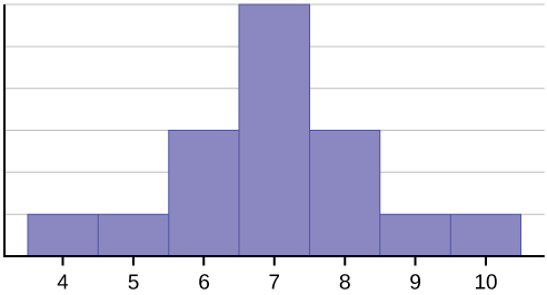
The histogram displays a symmetrical distribution of data. A distribution is symmetrical if a vertical line can be drawn at some point in the histogram such that the shape to the left and the right of the vertical line are mirror images of each other. The mean, the median, and the mode are each seven for these data. In a perfectly symmetrical distribution, the mean and the median are the same.
Skewed Distributions

The histogram for the data: 4; 5; 6; 6; 6; 7; 7; 7; 7; 8 is not symmetrical. The right-hand side seems "chopped off" compared to the left side. A distribution of this type is called skewed to the left because it is pulled out to the left.
The mean is 6.3, the median is 6.5, and the mode is seven. Notice that the mean is less than the median, and they are both less than the mode. The mean and the median both reflect the skewing, but the mean reflects it more so.
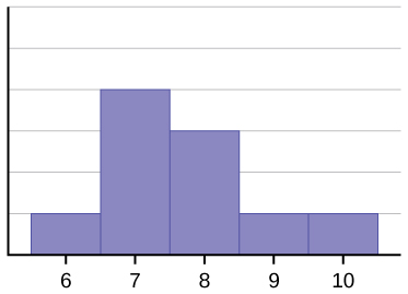
The histogram for the data: 6; 7; 7; 7; 7; 8; 8; 8; 9; 10, is also not symmetrical. It is skewed to the right.
The mean is 7.7, the median is 7.5, and the mode is seven. Of the three statistics, the mean is the largest, while the mode is the smallest. Again, the mean reflects the skewing the most.
For more information and examples see online textbook OpenStax Introductory Statistics pages 106-109.
“Introduction to Statistics” by OpenStax, used is licensed under a Creative Commons Attribution License 4.0 license