
2.5 Measures of Center of the Data
- Page ID
- 36467
\( \newcommand{\vecs}[1]{\overset { \scriptstyle \rightharpoonup} {\mathbf{#1}} } \)
\( \newcommand{\vecd}[1]{\overset{-\!-\!\rightharpoonup}{\vphantom{a}\smash {#1}}} \)
\( \newcommand{\id}{\mathrm{id}}\) \( \newcommand{\Span}{\mathrm{span}}\)
( \newcommand{\kernel}{\mathrm{null}\,}\) \( \newcommand{\range}{\mathrm{range}\,}\)
\( \newcommand{\RealPart}{\mathrm{Re}}\) \( \newcommand{\ImaginaryPart}{\mathrm{Im}}\)
\( \newcommand{\Argument}{\mathrm{Arg}}\) \( \newcommand{\norm}[1]{\| #1 \|}\)
\( \newcommand{\inner}[2]{\langle #1, #2 \rangle}\)
\( \newcommand{\Span}{\mathrm{span}}\)
\( \newcommand{\id}{\mathrm{id}}\)
\( \newcommand{\Span}{\mathrm{span}}\)
\( \newcommand{\kernel}{\mathrm{null}\,}\)
\( \newcommand{\range}{\mathrm{range}\,}\)
\( \newcommand{\RealPart}{\mathrm{Re}}\)
\( \newcommand{\ImaginaryPart}{\mathrm{Im}}\)
\( \newcommand{\Argument}{\mathrm{Arg}}\)
\( \newcommand{\norm}[1]{\| #1 \|}\)
\( \newcommand{\inner}[2]{\langle #1, #2 \rangle}\)
\( \newcommand{\Span}{\mathrm{span}}\) \( \newcommand{\AA}{\unicode[.8,0]{x212B}}\)
\( \newcommand{\vectorA}[1]{\vec{#1}} % arrow\)
\( \newcommand{\vectorAt}[1]{\vec{\text{#1}}} % arrow\)
\( \newcommand{\vectorB}[1]{\overset { \scriptstyle \rightharpoonup} {\mathbf{#1}} } \)
\( \newcommand{\vectorC}[1]{\textbf{#1}} \)
\( \newcommand{\vectorD}[1]{\overrightarrow{#1}} \)
\( \newcommand{\vectorDt}[1]{\overrightarrow{\text{#1}}} \)
\( \newcommand{\vectE}[1]{\overset{-\!-\!\rightharpoonup}{\vphantom{a}\smash{\mathbf {#1}}}} \)
\( \newcommand{\vecs}[1]{\overset { \scriptstyle \rightharpoonup} {\mathbf{#1}} } \)
\( \newcommand{\vecd}[1]{\overset{-\!-\!\rightharpoonup}{\vphantom{a}\smash {#1}}} \)
Learning Objectives
In this section, you will:
• Measure the centers of data, including mean, median, and mode.
The "center" of a data set is also a way of describing location. The two most widely used measures of the "center" of the data are the mean (average) and the median.
Mean and Median
Mean: add all data, divide by the total number of values.
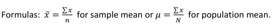
Median: middle value when the data are placed in order. If there is no middle value, find the mean of the two middle values.
• The median is generally a better measure of the center when there are extreme values or outliers because it is not affected by the precise numerical values of the outliers.
• You can quickly find the location of the median by using the expression (n + 1)/2.
Example 1
Consider the following data: 19; 18; 18; 25; 24; 32; 45; 29; 17; 18; 53; 30; 20; 21.
Find mean.
Find median.
Using the graphing calculator to find the mean and median.
• Clear list L1. Press STAT 4: ClrList. Enter 2nd 1 for list L1. Press ENTER.
• Enter data into the list editor. Press STAT 1: EDIT.
• Put the data values into list L1.
• Press STAT and arrow to CALC. Press 1:1-VarStats. Press 2nd 1 for L1 and then Calculate.
• Press the down and up arrow keys to scroll.
Example 2
AIDS data indicating the number of months a patient with AIDS lives after taking a new antibody drug are as follows (smallest to largest): 3; 4; 8; 8; 10; 11; 12; 13; 14; 15; 15; 16; 16; 17; 17; 18; 21; 22; 22; 24; 24; 25; 26; 26; 27; 27; 29; 29; 31; 32; 33; 33; 34; 34; 35; 37; 40; 44; 44; 47.
Calculate the mean and the median.
Mode
Another measure of the center is the mode. The is the most frequent value. There can be more than one mode in a data set as long as those values have the same frequency and that frequency is the highest. A data set with two modes is called bimodal.
Example 3
Statistics exam scores for 20 students are as follows: 50; 53; 59; 59; 63; 63; 72; 72; 72; 72; 72;
76; 78; 81; 83; 84; 84; 84; 90; 93.
Find the mode.
Calculating the Mean of Frequency Distribution
When only grouped data is available, you do not know the individual data values (we only know intervals and interval frequencies); therefore, you cannot compute an exact mean for the data set. What we must do is estimate the actual mean by calculating the mean of a frequency table.
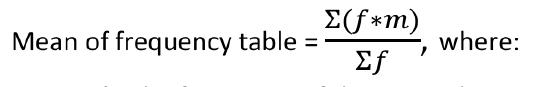
o f = the frequency of the interval
o m = the midpoint of the interval
Example 4
A frequency table displaying Professor Blount’s last statistic test is shown. Find the best estimate of the class mean.
| Grade Interval | Number of Students |
| 50.5-56.4 | 1 |
| 56.5-62.4 | 0 |
| 62.5-68.4 | 4 |
| 68.5-74.4 | 4 |
| 74.5-80.4 | 2 |
| 80.5-86.4 | 2 |
| 86.5-92.4 | 4 |
| 92.5-98.4 | 1 |
Using the graphing calculator to find the mean of grouped frequency tables.
• Clear list L1. Pres STAT 4:ClrList. Enter 2nd 1 for list L1. Press ENTER.
• Enter data into the list editor. Press STAT 1:EDIT.
• Put the midpoint values into list L1.
• Put the frequency values into list L2.
• Press STAT and arrow to CALC. Press 1:1-VarStats.
• List: Press 2nd 1 for L1.
• FreqList: Press 2nd 2 for L2. and then Calculate.
• Press the down and up arrow keys to scroll.
For more information and examples see online textbook OpenStax Introductory Statistics pages 100- 106.
“Introduction to Statistics” by OpenStax, used is licensed under a Creative Commons Attribution License 4.0 license