1.4.2: Observational Studies and Sampling Strategies
- Page ID
- 10910
\( \newcommand{\vecs}[1]{\overset { \scriptstyle \rightharpoonup} {\mathbf{#1}} } \)
\( \newcommand{\vecd}[1]{\overset{-\!-\!\rightharpoonup}{\vphantom{a}\smash {#1}}} \)
\( \newcommand{\id}{\mathrm{id}}\) \( \newcommand{\Span}{\mathrm{span}}\)
( \newcommand{\kernel}{\mathrm{null}\,}\) \( \newcommand{\range}{\mathrm{range}\,}\)
\( \newcommand{\RealPart}{\mathrm{Re}}\) \( \newcommand{\ImaginaryPart}{\mathrm{Im}}\)
\( \newcommand{\Argument}{\mathrm{Arg}}\) \( \newcommand{\norm}[1]{\| #1 \|}\)
\( \newcommand{\inner}[2]{\langle #1, #2 \rangle}\)
\( \newcommand{\Span}{\mathrm{span}}\)
\( \newcommand{\id}{\mathrm{id}}\)
\( \newcommand{\Span}{\mathrm{span}}\)
\( \newcommand{\kernel}{\mathrm{null}\,}\)
\( \newcommand{\range}{\mathrm{range}\,}\)
\( \newcommand{\RealPart}{\mathrm{Re}}\)
\( \newcommand{\ImaginaryPart}{\mathrm{Im}}\)
\( \newcommand{\Argument}{\mathrm{Arg}}\)
\( \newcommand{\norm}[1]{\| #1 \|}\)
\( \newcommand{\inner}[2]{\langle #1, #2 \rangle}\)
\( \newcommand{\Span}{\mathrm{span}}\) \( \newcommand{\AA}{\unicode[.8,0]{x212B}}\)
\( \newcommand{\vectorA}[1]{\vec{#1}} % arrow\)
\( \newcommand{\vectorAt}[1]{\vec{\text{#1}}} % arrow\)
\( \newcommand{\vectorB}[1]{\overset { \scriptstyle \rightharpoonup} {\mathbf{#1}} } \)
\( \newcommand{\vectorC}[1]{\textbf{#1}} \)
\( \newcommand{\vectorD}[1]{\overrightarrow{#1}} \)
\( \newcommand{\vectorDt}[1]{\overrightarrow{\text{#1}}} \)
\( \newcommand{\vectE}[1]{\overset{-\!-\!\rightharpoonup}{\vphantom{a}\smash{\mathbf {#1}}}} \)
\( \newcommand{\vecs}[1]{\overset { \scriptstyle \rightharpoonup} {\mathbf{#1}} } \)
\( \newcommand{\vecd}[1]{\overset{-\!-\!\rightharpoonup}{\vphantom{a}\smash {#1}}} \)
\(\newcommand{\avec}{\mathbf a}\) \(\newcommand{\bvec}{\mathbf b}\) \(\newcommand{\cvec}{\mathbf c}\) \(\newcommand{\dvec}{\mathbf d}\) \(\newcommand{\dtil}{\widetilde{\mathbf d}}\) \(\newcommand{\evec}{\mathbf e}\) \(\newcommand{\fvec}{\mathbf f}\) \(\newcommand{\nvec}{\mathbf n}\) \(\newcommand{\pvec}{\mathbf p}\) \(\newcommand{\qvec}{\mathbf q}\) \(\newcommand{\svec}{\mathbf s}\) \(\newcommand{\tvec}{\mathbf t}\) \(\newcommand{\uvec}{\mathbf u}\) \(\newcommand{\vvec}{\mathbf v}\) \(\newcommand{\wvec}{\mathbf w}\) \(\newcommand{\xvec}{\mathbf x}\) \(\newcommand{\yvec}{\mathbf y}\) \(\newcommand{\zvec}{\mathbf z}\) \(\newcommand{\rvec}{\mathbf r}\) \(\newcommand{\mvec}{\mathbf m}\) \(\newcommand{\zerovec}{\mathbf 0}\) \(\newcommand{\onevec}{\mathbf 1}\) \(\newcommand{\real}{\mathbb R}\) \(\newcommand{\twovec}[2]{\left[\begin{array}{r}#1 \\ #2 \end{array}\right]}\) \(\newcommand{\ctwovec}[2]{\left[\begin{array}{c}#1 \\ #2 \end{array}\right]}\) \(\newcommand{\threevec}[3]{\left[\begin{array}{r}#1 \\ #2 \\ #3 \end{array}\right]}\) \(\newcommand{\cthreevec}[3]{\left[\begin{array}{c}#1 \\ #2 \\ #3 \end{array}\right]}\) \(\newcommand{\fourvec}[4]{\left[\begin{array}{r}#1 \\ #2 \\ #3 \\ #4 \end{array}\right]}\) \(\newcommand{\cfourvec}[4]{\left[\begin{array}{c}#1 \\ #2 \\ #3 \\ #4 \end{array}\right]}\) \(\newcommand{\fivevec}[5]{\left[\begin{array}{r}#1 \\ #2 \\ #3 \\ #4 \\ #5 \\ \end{array}\right]}\) \(\newcommand{\cfivevec}[5]{\left[\begin{array}{c}#1 \\ #2 \\ #3 \\ #4 \\ #5 \\ \end{array}\right]}\) \(\newcommand{\mattwo}[4]{\left[\begin{array}{rr}#1 \amp #2 \\ #3 \amp #4 \\ \end{array}\right]}\) \(\newcommand{\laspan}[1]{\text{Span}\{#1\}}\) \(\newcommand{\bcal}{\cal B}\) \(\newcommand{\ccal}{\cal C}\) \(\newcommand{\scal}{\cal S}\) \(\newcommand{\wcal}{\cal W}\) \(\newcommand{\ecal}{\cal E}\) \(\newcommand{\coords}[2]{\left\{#1\right\}_{#2}}\) \(\newcommand{\gray}[1]{\color{gray}{#1}}\) \(\newcommand{\lgray}[1]{\color{lightgray}{#1}}\) \(\newcommand{\rank}{\operatorname{rank}}\) \(\newcommand{\row}{\text{Row}}\) \(\newcommand{\col}{\text{Col}}\) \(\renewcommand{\row}{\text{Row}}\) \(\newcommand{\nul}{\text{Nul}}\) \(\newcommand{\var}{\text{Var}}\) \(\newcommand{\corr}{\text{corr}}\) \(\newcommand{\len}[1]{\left|#1\right|}\) \(\newcommand{\bbar}{\overline{\bvec}}\) \(\newcommand{\bhat}{\widehat{\bvec}}\) \(\newcommand{\bperp}{\bvec^\perp}\) \(\newcommand{\xhat}{\widehat{\xvec}}\) \(\newcommand{\vhat}{\widehat{\vvec}}\) \(\newcommand{\uhat}{\widehat{\uvec}}\) \(\newcommand{\what}{\widehat{\wvec}}\) \(\newcommand{\Sighat}{\widehat{\Sigma}}\) \(\newcommand{\lt}{<}\) \(\newcommand{\gt}{>}\) \(\newcommand{\amp}{&}\) \(\definecolor{fillinmathshade}{gray}{0.9}\)Observational Studies
Generally, data in observational studies are collected only by monitoring what occurs, what occurs, while experiments require the primary explanatory variable in a study be assigned for each subject by the researchers. Making causal conclusions based on experiments is often reasonable. However, making the same causal conclusions based on observational data can be treacherous and is not recommended. Thus, observational studies are generally only sufficient to show associations.
Exercise \(\PageIndex{1}\)
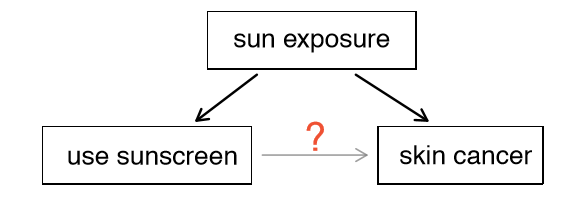
Suppose an observational study tracked sunscreen use and skin cancer, and it was found that the more sunscreen someone used, the more likely the person was to have skin cancer. Does this mean sunscreen causes skin cancer?
Solution
No. See the paragraph following the exercise for an explanation.
Some previous research tells us that using sunscreen actually reduces skin cancer risk, so maybe there is another variable that can explain this hypothetical association between sunscreen usage and skin cancer. One important piece of information that is absent is sun exposure. If someone is out in the sun all day, she is more likely to use sunscreen and more likely to get skin cancer. Exposure to the sun is unaccounted for in the simple investigation.

Sun exposure is what is called a confounding variable (also called a lurking variable, confounding factor, or a confounder), which is a variable that is correlated with both the explanatory and response variables. While one method to justify making causal conclusions from observational studies is to exhaust the search for confounding variables, there is no guarantee that all confounding variables can be examined or measured. In the same way, the county data set is an observational study with confounding variables, and its data cannot easily be used to make causal conclusions.
Exercise \(\PageIndex{2}\)
Figure 1.9 shows a negative association between the homeownership rate and the percentage of multi-unit structures in a county. However, it is unreasonable to conclude that there is a causal relationship between the two variables. Suggest one or more other variables that might explain the relationship visible in Figure 1.9.
Solution
Answers will vary. Population density may be important. If a county is very dense, then this may require a larger fraction of residents to live in multi-unit structures. Additionally, the high density may contribute to increases in property value, making homeownership infeasible for many residents.
Observational studies come in two forms: prospective and retrospective studies. A prospective study identifies individuals and collects information as events unfold. For instance, medical researchers may identify and follow a group of similar individuals over many years to assess the possible influences of behavior on cancer risk. One example of such a study is The Nurses Health Study, started in 1976 and expanded in 1989. This prospective study recruits registered nurses and then collects data from them using questionnaires. Retrospective studies collect data after events have taken place, e.g. researchers may review past events in medical records. Some data sets, such as county, may contain both rospectively- and retrospectively-collected variables. Local governments prospectively collect some variables as events unfolded (e.g. retails sales) while the federal government retrospectively collected others during the 2010 census (e.g. county population counts).
Three Sampling Methods
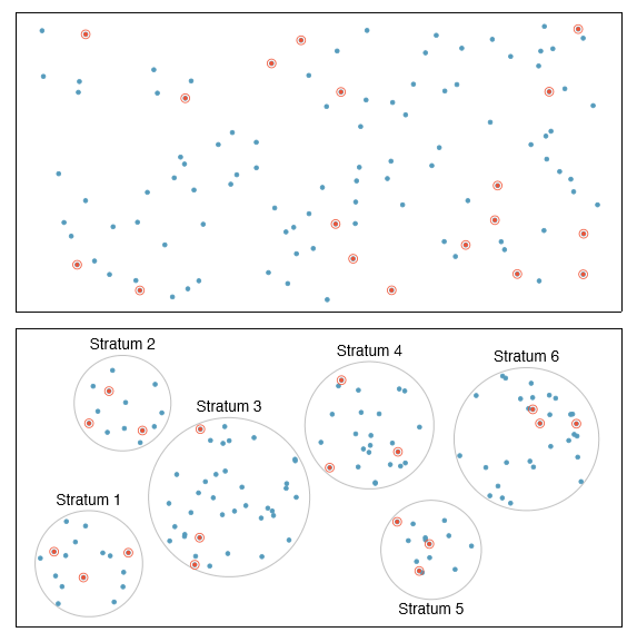
Almost all statistical methods are based on the notion of implied randomness. If observational data are not collected in a random framework from a population, these statistical methods are not reliable. Here we consider three random sampling techniques: simple, stratified, and cluster sampling. Figure 1.14 provides a graphical representation of these techniques.
Simple random sampling is probably the most intuitive form of random sampling. Consider the salaries of Major League Baseball (MLB) players, where each player is a member of one of the league's 30 teams. To take a simple random sample of 120 baseball players and their salaries from the 2010 season, we could write the names of that season's 828 players onto slips of paper, drop the slips into a bucket, shake the bucket around until we are sure the names are all mixed up, then draw out slips until we have the sample of 120 players. In general, a sample is referred to as "simple random" if each case in the population has an equal chance of being included in the nal sample and knowing that a case is included in a sample does not provide useful information about which other cases are included.
Stratified sampling is a divide-and-conquer sampling strategy. The population is divided into groups called strata. The strata are chosen so that similar cases are grouped together, then a second sampling method, usually simple random sampling, is employed within each stratum. In the baseball salary example, the teams could represent the strata; some teams have a lot more money (we're looking at you, Yankees). Then we might randomly sample 4 players from each team for a total of 120 players.

Figure 1.14: Examples of simple random, stratified, and cluster sampling. In the top panel, simple random sampling was used to randomly select the 18 cases. In the middle panel, stratified sampling was used: cases were grouped into strata, and then simple random sampling was employed within each stratum. In the bottom panel, cluster sampling was used, where data were binned into nine clusters, three of the clusters were randomly selected, and six cases were randomly sampled in each of these clusters.
Stratified sampling is especially useful when the cases in each stratum are very similar with respect to the outcome of interest. The downside is that analyzing data from a stratified sample is a more complex task than analyzing data from a simple random sample. The analysis methods introduced in this book would need to be extended to analyze data collected using stratified sampling.
Example \(\PageIndex{1}\)
Why would it be good for cases within each stratum to be very similar?
Solution
We might get a more stable estimate for the subpopulation in a stratum if the cases are very similar. These improved estimates for each subpopulation will help us build a reliable estimate for the full population.
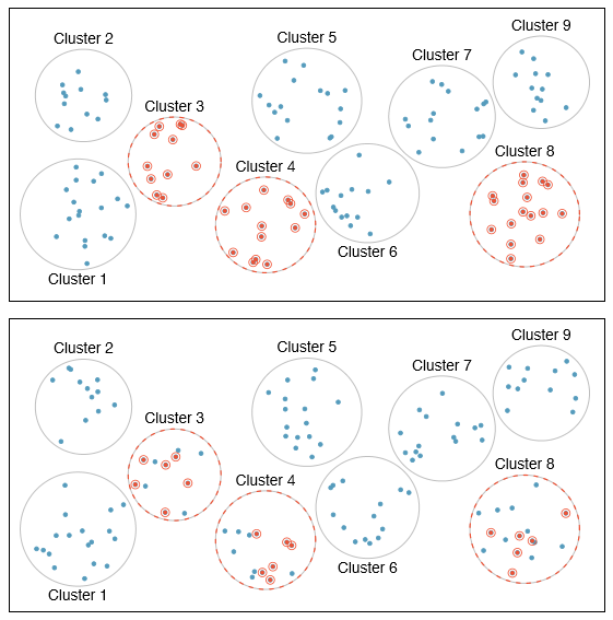
A cluster sample is employed by taking all of the members from some of the groups. That is, we break up the population into many groups, called clusters. Then we sample a fixed number of clusters and use all the members within each cluster. If the population is large, instead of taking all members of the selected clusters, we can perform a simple random sample within the clusters. This technique is similar to stratified sampling in its process, except that there is no requirement in cluster sampling to sample from every cluster. Stratified sampling requires observations be sampled from every stratum.

Figure 1.15: Examples of cluster and multistage sampling. In the top panel, cluster sampling was used. Here, data were binned into nine clusters, three of these clusters were sampled, and all observations within these three cluster were included in the sample. In the bottom panel, multistage sampling was used. It differs from cluster sampling in that of the clusters selected, we randomly select a subset of each cluster to be included in the sample.
Sometimes cluster sampling can be a more economical random sampling technique than the alternatives. Also, unlike stratified sampling, cluster sampling is most helpful when there is a lot of case-to-case variability within a cluster but the clusters themselves don't look very different from one another. For example, if neighborhoods represented clusters, then this sampling method works best when the neighborhoods are very diverse. A downside of cluster sampling is that more advanced analysis techniques are typically required, though the methods in this book can be extended to handle such data.
Example \(\PageIndex{3}\)
Suppose we are interested in estimating the malaria rate in a densely tropical portion of rural Indonesia. We learn that there are 30 villages in that part of the Indonesian jungle, each more or less similar to the next. Our goal is to test 150 individuals for malaria. What sampling method should be employed?
Solution
A simple random sample would likely draw individuals from all 30 villages, which could make data collection extremely expensive. Stratified sampling would be a challenge since it is unclear how we would build strata of similar individuals. However, cluster sampling seems like a very good idea. First, we might randomly select half the villages, then randomly select 10 people from each. This would probably reduce our data collection costs substantially in comparison to a simple random sample and would still give us reliable information.
Contributors and Attributions
David M Diez (Google/YouTube), Christopher D Barr (Harvard School of Public Health), Mine Çetinkaya-Rundel (Duke University)


