Write an Equation of a Line
- Page ID
- 29783

Plotting Points and Graphing Lines
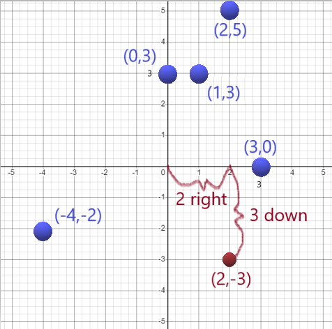
Plot the points (0,3),(3,0),(1,3),(2,5),(-4,-2)
|
|
\((x,y)\) means the following: The first number represents the number of units right (if positive) or left (if negative) that you move in the \(x\)-direction. From that point on the \(x\)-axis, go up (if positive) or down (if negative) the number of units in the
\((2,3)\) means starting at the middle, go two right and 3 down |
Evaluate the following linear equation for the given values.
|
\(x\) |
|
\(y=-2x-3\) |
Substitute each \(x\)-value into \(-2x-3\) to find the corresponding \(y\)-value |
|
-3 |
|
\(y=-2(-3)-3=3\) |
|
|
7 |
|
\(y=-2(-7)-3=3-17\) |
|
|
6 |
|
\(y=-2(-6)-3=3-15\) |
|
|
4 |
|
\(y=-2(4)-3=-11\) |
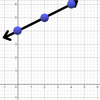
Fill in the table below for the equation. Then graph the line on the grid by selecting two of the points from your table.
\(y=\frac{1}{2}x+4\)
|
\(x\) |
\(y\) |
|
Next, plot points: (0,4) (2,5) (4,6) and then connect the dots |
|
0 |
4 |
\(y=\frac{1}{2}(0)+4=4\) |
|
|
2 |
5 |
\(y=\frac{1}{2}(2)+4=5\) |
|
|
4 |
6 |
\(y=\frac{1}{2}(6)+4=6\) |
Plotting Points and Lines
Thus far, we have used one dimensional number lines as a way to visualize ranges of values for a single variable ![]() . In this section, we are going to be concerned with values of two different variables represented by
. In this section, we are going to be concerned with values of two different variables represented by ![]() and
and ![]() . When plotting values for two different variables at the same time, instead of having a one dimensional horizontal number line, we have two intersecting number lines that are perpendicular to each other.
. When plotting values for two different variables at the same time, instead of having a one dimensional horizontal number line, we have two intersecting number lines that are perpendicular to each other.
|
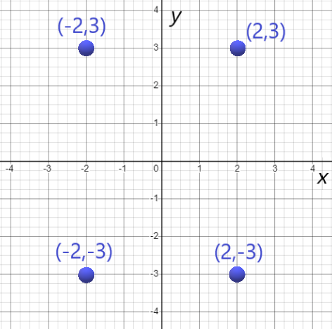
The horizontal axis represents the scale for the first variable, \(x\). The vertical axis represents the scale for the second variable \(y\). The \((x,y)\) values are plotted by first going \(x\) units left or right along the horizontal axis and then starting from that point \(y\) units up or down. |
|
Plotting points is very useful to graph lines. In this section we will see that lines have useful applications in statistics.
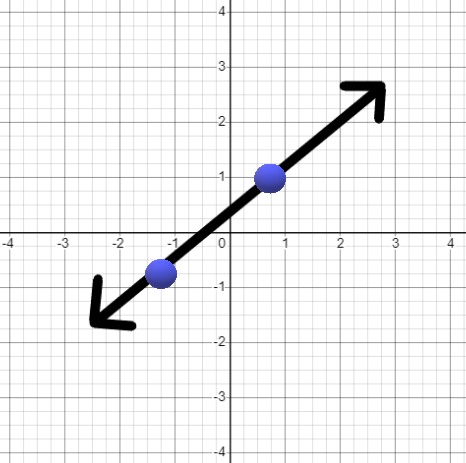
Lines are characterized by their slopes.
|
A line with positive slope slopes up to the right
|
|
|
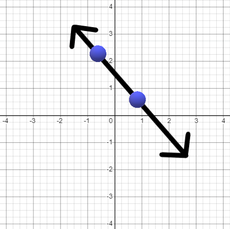
A line with negative slope slopes up to the left.
|
|
|
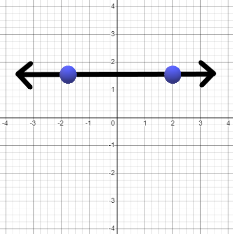
A line with 0 slope is flat or horizontal.
|
|
Slope
The equation of a line can be found using any two points on the line. To find the equation of a line using two points first find the slope. The slope measures the degree of slant of the line and is given by
\(m=\frac{y_2 - y_1}{x_2-x_1}\) where \((x_1,y_1)\) and \((x_2,y_2)\) are any two different \((x,y)\) pairs on the line.
Example: If a line contains the two points \((-1,3)\) and \((3,11)\) then \(x_1=-1, y_1=3, x_2=3, y_2=11\) and the slope is:
\(m=\frac{y_2-y_1}{x_2-x_1}=\frac{11-3}{3-1}=\frac{8}{4}=2\)
Given the slope \(m\) and any point \((x_1,y_1)\) on the line one can find the equation of the line in slope intercept form: \(y=mx+b\) by doing the following steps:
1. Plug in ![]() , \(m\), \(x_1\) and \(y_1\) into \(y-y_1=m(x-x_1)\)
, \(m\), \(x_1\) and \(y_1\) into \(y-y_1=m(x-x_1)\)
In our example, \(m=2\) and we could use either point as \((x_1,y_1)\) . Let’s use \((-1,3)\). So
\(y-3=2(x- -1)\)
2. Solve for \(y\) and eliminate parentheses to get it into the form \(y=mx+b\).
\(y-3 = 2(x - -1)\)
\(y-3 = 2(x + 1)\)
\(y-3 = 2x + 2\)
+3 +3
\(y = 2x+5\) Note that \(m=2\) and \(b = 5 \)
\(m\) is the slope: \(m=2\)
\(b\) is the \(y\)-intersect: \(b = 5\)
means the line crosses the -\(x\)-axis at \((0,5)\).
Finding the Slope of a Line and \(y\)-Intercept
Slope can be calculated by using any two points on the line as the difference in the \(y\)-values divided by the difference in the \(x\)-values:
\[m=\frac{y_2-y_1}{x_2-x_1}\]
Example: Given the points \((8,-9)\) and \((7,-1)\).
Here: \(x_1=8, y_1=-9, x_2=7, y_2=-1\)
Find the slope.
\(m=\frac{y_2-y_1}{x_2-x_1}=\frac{-1- -9}{7-8}=\frac{8}{-1}=-8\)
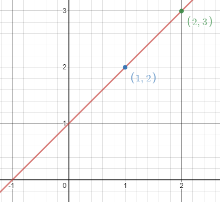
Example: Find the slope of the line shown below
|
|
Find the \((x,y)\) values for two different points on the line.
For example: \((x_1,y_1)=(2,3)\) & \((x_2,y_2) = (1,2)\)
Slope \(m=\frac{y_2-y_1}{x_2-x_1)=\frac{2-3}{1-2}=\frac{-1}{-1}=1\)
Slope = 1 |
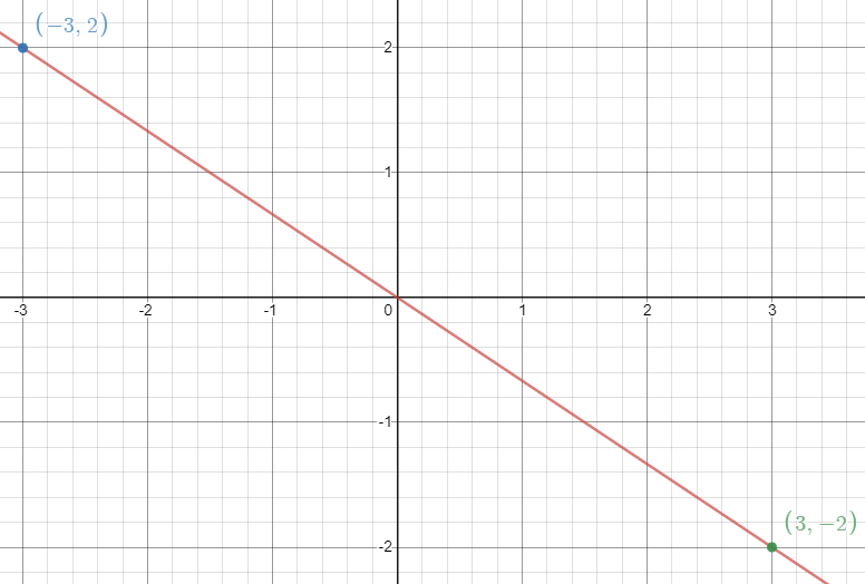
Example: Find the slope of the line shown below.
|
|
Again, find the \((x,y)\) for two different points:
For example: \((x_1,y_1)=(-3,2)\) & \((x_2,y_2) = (3,-2)\)
Slope \(m=\frac{y_2-y_1}{x_2-x_1}=\frac{-2-2}{3- -3}=\frac{-4}{6}=\frac{-2}{3}\) (reduced)
Slope = \(\frac{-2}{3}\) |