10.4: Comparing Two Independent Population Proportions
- Page ID
- 20423
\( \newcommand{\vecs}[1]{\overset { \scriptstyle \rightharpoonup} {\mathbf{#1}} } \)
\( \newcommand{\vecd}[1]{\overset{-\!-\!\rightharpoonup}{\vphantom{a}\smash {#1}}} \)
\( \newcommand{\id}{\mathrm{id}}\) \( \newcommand{\Span}{\mathrm{span}}\)
( \newcommand{\kernel}{\mathrm{null}\,}\) \( \newcommand{\range}{\mathrm{range}\,}\)
\( \newcommand{\RealPart}{\mathrm{Re}}\) \( \newcommand{\ImaginaryPart}{\mathrm{Im}}\)
\( \newcommand{\Argument}{\mathrm{Arg}}\) \( \newcommand{\norm}[1]{\| #1 \|}\)
\( \newcommand{\inner}[2]{\langle #1, #2 \rangle}\)
\( \newcommand{\Span}{\mathrm{span}}\)
\( \newcommand{\id}{\mathrm{id}}\)
\( \newcommand{\Span}{\mathrm{span}}\)
\( \newcommand{\kernel}{\mathrm{null}\,}\)
\( \newcommand{\range}{\mathrm{range}\,}\)
\( \newcommand{\RealPart}{\mathrm{Re}}\)
\( \newcommand{\ImaginaryPart}{\mathrm{Im}}\)
\( \newcommand{\Argument}{\mathrm{Arg}}\)
\( \newcommand{\norm}[1]{\| #1 \|}\)
\( \newcommand{\inner}[2]{\langle #1, #2 \rangle}\)
\( \newcommand{\Span}{\mathrm{span}}\) \( \newcommand{\AA}{\unicode[.8,0]{x212B}}\)
\( \newcommand{\vectorA}[1]{\vec{#1}} % arrow\)
\( \newcommand{\vectorAt}[1]{\vec{\text{#1}}} % arrow\)
\( \newcommand{\vectorB}[1]{\overset { \scriptstyle \rightharpoonup} {\mathbf{#1}} } \)
\( \newcommand{\vectorC}[1]{\textbf{#1}} \)
\( \newcommand{\vectorD}[1]{\overrightarrow{#1}} \)
\( \newcommand{\vectorDt}[1]{\overrightarrow{\text{#1}}} \)
\( \newcommand{\vectE}[1]{\overset{-\!-\!\rightharpoonup}{\vphantom{a}\smash{\mathbf {#1}}}} \)
\( \newcommand{\vecs}[1]{\overset { \scriptstyle \rightharpoonup} {\mathbf{#1}} } \)
\( \newcommand{\vecd}[1]{\overset{-\!-\!\rightharpoonup}{\vphantom{a}\smash {#1}}} \)
\(\newcommand{\avec}{\mathbf a}\) \(\newcommand{\bvec}{\mathbf b}\) \(\newcommand{\cvec}{\mathbf c}\) \(\newcommand{\dvec}{\mathbf d}\) \(\newcommand{\dtil}{\widetilde{\mathbf d}}\) \(\newcommand{\evec}{\mathbf e}\) \(\newcommand{\fvec}{\mathbf f}\) \(\newcommand{\nvec}{\mathbf n}\) \(\newcommand{\pvec}{\mathbf p}\) \(\newcommand{\qvec}{\mathbf q}\) \(\newcommand{\svec}{\mathbf s}\) \(\newcommand{\tvec}{\mathbf t}\) \(\newcommand{\uvec}{\mathbf u}\) \(\newcommand{\vvec}{\mathbf v}\) \(\newcommand{\wvec}{\mathbf w}\) \(\newcommand{\xvec}{\mathbf x}\) \(\newcommand{\yvec}{\mathbf y}\) \(\newcommand{\zvec}{\mathbf z}\) \(\newcommand{\rvec}{\mathbf r}\) \(\newcommand{\mvec}{\mathbf m}\) \(\newcommand{\zerovec}{\mathbf 0}\) \(\newcommand{\onevec}{\mathbf 1}\) \(\newcommand{\real}{\mathbb R}\) \(\newcommand{\twovec}[2]{\left[\begin{array}{r}#1 \\ #2 \end{array}\right]}\) \(\newcommand{\ctwovec}[2]{\left[\begin{array}{c}#1 \\ #2 \end{array}\right]}\) \(\newcommand{\threevec}[3]{\left[\begin{array}{r}#1 \\ #2 \\ #3 \end{array}\right]}\) \(\newcommand{\cthreevec}[3]{\left[\begin{array}{c}#1 \\ #2 \\ #3 \end{array}\right]}\) \(\newcommand{\fourvec}[4]{\left[\begin{array}{r}#1 \\ #2 \\ #3 \\ #4 \end{array}\right]}\) \(\newcommand{\cfourvec}[4]{\left[\begin{array}{c}#1 \\ #2 \\ #3 \\ #4 \end{array}\right]}\) \(\newcommand{\fivevec}[5]{\left[\begin{array}{r}#1 \\ #2 \\ #3 \\ #4 \\ #5 \\ \end{array}\right]}\) \(\newcommand{\cfivevec}[5]{\left[\begin{array}{c}#1 \\ #2 \\ #3 \\ #4 \\ #5 \\ \end{array}\right]}\) \(\newcommand{\mattwo}[4]{\left[\begin{array}{rr}#1 \amp #2 \\ #3 \amp #4 \\ \end{array}\right]}\) \(\newcommand{\laspan}[1]{\text{Span}\{#1\}}\) \(\newcommand{\bcal}{\cal B}\) \(\newcommand{\ccal}{\cal C}\) \(\newcommand{\scal}{\cal S}\) \(\newcommand{\wcal}{\cal W}\) \(\newcommand{\ecal}{\cal E}\) \(\newcommand{\coords}[2]{\left\{#1\right\}_{#2}}\) \(\newcommand{\gray}[1]{\color{gray}{#1}}\) \(\newcommand{\lgray}[1]{\color{lightgray}{#1}}\) \(\newcommand{\rank}{\operatorname{rank}}\) \(\newcommand{\row}{\text{Row}}\) \(\newcommand{\col}{\text{Col}}\) \(\renewcommand{\row}{\text{Row}}\) \(\newcommand{\nul}{\text{Nul}}\) \(\newcommand{\var}{\text{Var}}\) \(\newcommand{\corr}{\text{corr}}\) \(\newcommand{\len}[1]{\left|#1\right|}\) \(\newcommand{\bbar}{\overline{\bvec}}\) \(\newcommand{\bhat}{\widehat{\bvec}}\) \(\newcommand{\bperp}{\bvec^\perp}\) \(\newcommand{\xhat}{\widehat{\xvec}}\) \(\newcommand{\vhat}{\widehat{\vvec}}\) \(\newcommand{\uhat}{\widehat{\uvec}}\) \(\newcommand{\what}{\widehat{\wvec}}\) \(\newcommand{\Sighat}{\widehat{\Sigma}}\) \(\newcommand{\lt}{<}\) \(\newcommand{\gt}{>}\) \(\newcommand{\amp}{&}\) \(\definecolor{fillinmathshade}{gray}{0.9}\)When conducting a hypothesis test that compares two independent population proportions, the following characteristics should be present:
- The two independent samples are simple random samples that are independent.
- The number of successes is at least five, and the number of failures is at least five, for each of the samples.
- Growing literature states that the population must be at least ten or 20 times the size of the sample. This keeps each population from being over-sampled and causing incorrect results.
Comparing two proportions, like comparing two means, is common. If two estimated proportions are different, it may be due to a difference in the populations or it may be due to chance. A hypothesis test can help determine if a difference in the estimated proportions reflects a difference in the population proportions.
The difference of two proportions follows an approximate normal distribution. Generally, the null hypothesis states that the two proportions are the same. That is, \(H_{0}: p_{A} = p_{B}\). To conduct the test, we use a pooled proportion, \(p_{c}\).
The pooled proportion is calculated as follows:
\[p_{c} = \dfrac{x_{A} + x_{B}}{n_{A} + n_{B}}\]
The distribution for the differences is:
\[\hat{p}_{A} - \hat{p}_{B} \sim N\left[0, \sqrt{p_{c}(1 - p_{c})\left(\dfrac{1}{n_{A}} + \dfrac{1}{n_{B}}\right)}\right]\]
The test statistic (z-score) is:
\[z = \dfrac{( \hat{p}_{A} - \hat{p}_{B}) - (p_{A} - p_{B})}{\sqrt{p_{c}(1 - p_{c})\left(\dfrac{1}{n_{A}} + \dfrac{1}{n_{B}}\right)}}\]
Two Proportions Calculator
Enter in the sample sizes and number of successes for each sample, the tail type and the confidence level and hit Calculate and the test statistic, t, the p-value, p, the confidence interval's lower bound, LB, and the upper bound, UB will be shown. Be sure to enter the confidence level as a decimal, e.g., 95% has a CL of 0.95.
| Sample Size | Number of Successes | |
| First Sample | ||
| Second Sample |
|
|
| z: | p: | LB: | UB: |
Example \(\PageIndex{1}\)
Two types of medication for hives are being tested to determine if there is a difference in the proportions of adult patient reactions. Twenty out of a random sample of 200 adults given medication A still had hives 30 minutes after taking the medication. Twelve out of another random sample of 200 adults given medication B still had hives 30 minutes after taking the medication. Test at a 1% level of significance.
Answer
The problem asks for a difference in proportions, making it a test of two proportions.
Let \(A\) and \(B\) be the subscripts for medication A and medication B, respectively. Then \(p_{A}\) and \(p_{B}\) are the desired population proportions.
Random Variable:\( \hat{p}_{A} – \hat{p}_{B} =\) difference in the proportions of adult patients who did not react after 30 minutes to medication A and to medication B.
\(H_{0}: p_{A} = p_{B}\) or \(p_{A} - p_{B} = 0\)
\(H_{a}: p_{A} \neq p_{B}\) or \(p_{A} - p_{B} \neq 0\)
The words "is a difference" tell you the test is two-tailed.
Distribution for the test: Since this is a test of two binomial population proportions, the distribution is normal:
\[p_{c} = \dfrac{x_{A} + x_{B}}{n_{A} + n_{B}} = \dfrac{20 + 12}{200 + 200} = 0.08, 1 - p_{c} = 0.92\]
\[ \hat{p}_{A} - \hat{p}_{B} \sim N\left[0, \sqrt{(0.08)(0.92)\left(\dfrac{1}{200} + \dfrac{1}{200}\right)}\right]\]
\( \hat{p}_{A} - \hat{p}_{B}\) follows an approximate normal distribution.
Calculate the p-value using the normal distribution: \(p\text{-value} = 0.1404\).
Estimated proportion for group A: \( \hat{p}_{A} = \dfrac{x_{A}}{n_{A}} = \dfrac{20}{200} = 0.1\)
Estimated proportion for group B: \( \hat{p}_{B} = \dfrac{x_{B}}{n_{B}} = \dfrac{12}{200} = 0.06\)
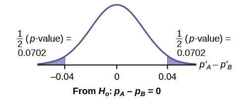
Graph:

\(\hat{p}_{A} - \hat{p}_{B} = 0.1 – 0.06 = 0.04\).
Half the \(p\text{-value}\) is below -0.04, and half is above 0.04.
Compare \(\alpha\) and the \(p\text{-value}: \alpha = 0.01\) and the \(p\text{-value} = 0.1404\). \(\alpha < p\text{-value}\).
Make a decision: Since \(\alpha < p\text{-value}\), do not reject \(H_{0}\).
Conclusion: At a 1% level of significance, from the sample data, there is not sufficient evidence to conclude that there is a difference in the proportions of adult patients who did not react after 30 minutes to medication A and medication B.
To use the Two Proportions calculator:
First Sample Sample Size = 200, First Sample Number of Successes = 20
Second Sample Sample Size = 200, Second Sample Number of Successes = 12
Check "\(\neq\)" and hit Calculate. The p-value is p = 0.1404 and the test statistic is 1.47.
Exercise \(\PageIndex{2}\)
Two types of valves are being tested to determine if there is a difference in pressure tolerances. Fifteen out of a random sample of 100 of Valve A cracked under 4,500 psi. Six out of a random sample of 100 of Valve B cracked under 4,500 psi. Test at a 5% level of significance.
Answer
The \(p\text{-value}\) is 0.0379, so we can reject the null hypothesis. At the 5% significance level, the data support that there is a difference in the pressure tolerances between the two valves.
Example \(\PageIndex{3}\): Sexting
A research study was conducted about gender differences in “sexting.” The researcher believed that the proportion of girls involved in “sexting” is less than the proportion of boys involved. The data collected in the spring of 2010 among a random sample of middle and high school students in a large school district in the southern United States is summarized in Table. Is the proportion of girls sending sexts less than the proportion of boys “sexting?” Test at a 1% level of significance.
| Males | Females | |
|---|---|---|
| Sent “sexts” | 183 | 156 |
| Total number surveyed | 2231 | 2169 |
Answer
This is a test of two population proportions. Let M and F be the subscripts for males and females. Then \(p_{M}\) and \(p_{F}\) are the desired population proportions.
Random variable:\(\hat{p}_{F} - \hat{p}_{M} =\) difference in the proportions of males and females who sent “sexts.”
\(H_{0}: p_{F} = p_{M} \) or \(H_{0}: p_{F} - p_{M} = 0\)
\(H_{a}: p_{F} < p_{M} \) or \(H_{a}: p_{F} - p_{M} < 0\)
The words "less than" tell you the test is left-tailed.
Distribution for the test: Since this is a test of two population proportions, the distribution is normal:
\[p_{C} = \dfrac{x_{F} + x_{M}}{n_{F} + n_{M}} = \dfrac{156 + 183}{2169 + 2231} = 0.077\]
\[1 - p_{C} = 0.923\]
Therefore,
\[\hat{p}_{F} - \hat{p}_{M} \sim N\left(0, \sqrt{(0.077)(0.923)\left(\dfrac{1}{2169} + \dfrac{1}{2231}\right)}\right)\]
\(\hat{p}_{F} – \hat{p}_{M}\) follows an approximate normal distribution.
Calculate the \(p\text{-value}\) using the normal distribution:
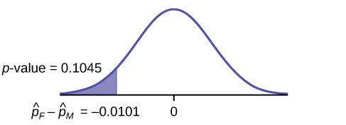
\(p\text{-value} = 0.1045\)
Estimated proportion for females: 0.0719
Estimated proportion for males: 0.082
Graph:

Decision: Since \(\alpha < p\text{-value}\), Do not reject \(H_{0}\)
Conclusion: At the 1% level of significance, from the sample data, there is not sufficient evidence to conclude that the proportion of girls sending “sexts” is less than the proportion of boys sending “sexts.”
To use the Two Proportions calculator:
First Sample Sample Size = 2169, First Sample Number of Successes = 156
Second Sample Sample Size = 2231, Second Sample Number of Successes = 183
Check "<" and hit Calculate. The \(p\text{-value}\) is \(p = 0.1045\) and the test statistic is \(z = -1.256\).
Example \(\PageIndex{4}\)
Researchers conducted a study of smartphone use among adults. A cell phone company claimed that iPhone smartphones are more popular with whites (non-Hispanic) than with African Americans. The results of the survey indicate that of the 232 African American cell phone owners randomly sampled, 5% have an iPhone. Of the 1,343 white cell phone owners randomly sampled, 10% own an iPhone. Test at the 5% level of significance. Is the proportion of white iPhone owners greater than the proportion of African American iPhone owners?
Answer
This is a test of two population proportions. Let W and A be the subscripts for the whites and African Americans. Then pW and pA are the desired population proportions.
Random variable: \(\hat{p}_{W} – \hat{p}_{A} =\) difference in the proportions of Android and iPhone users.
\(H_{0}: p_{W} = p_{A} \) or \(H_{0}: p_{W} – p_{A} = 0\)
\(H_{a}: p_{W} > p_{A}\) or \( H_{a}: p_{W} – p_{A} > 0\)
The words "more popular" indicate that the test is right-tailed.
Distribution for the test: The distribution is approximately normal:
\[p_{C} = \dfrac{x_{W} + x_{A}}{n_{W} + n_{A}} = \dfrac{134 + 12}{1343 + 232} = 0.0927\]
\[1 - p_{C} = 0.9073\]
Therefore,
\[\hat{p}_{W} - \hat{p}_{A} \sim N\left(0, \sqrt{(0.0927)(0.9073)\left(\dfrac{1}{1343} + \dfrac{1}{232}\right)}\right)\]
\(\hat{p}_{W} - \hat{p}_{A}\) follows an approximate normal distribution.
Calculate the \(p\text{-value}\) using the normal distribution:
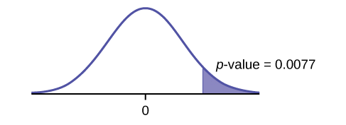
\(p\text{-value} = 0.0077\)
Estimated proportion for group A: 0.10
Estimated proportion for group B: 0.05
Graph:

Decision: Since \(\alpha > p\text{-value}\), reject the \(H_{0}\).
Conclusion: At the 5% level of significance, from the sample data, there is sufficient evidence to conclude that a larger proportion of white cell phone owners use iPhones than African Americans.
To use the Two Proportions calculator:
First Sample Sample Size = 1343, First Sample Number of Successes = 135
Second Sample Sample Size = 232, Second Sample Number of Successes = 12
Check ">" and hit Calculate. The \(p\text{-value}\) is \(p = 0.0092\) and the test statistic is \(z = 2.33\).
Example \(\PageIndex{5}\)
A concerned group of citizens wanted to know if the proportion of forcible rapes in Texas was different in 2011 than in 2010. Their research showed that of the 113,231 violent crimes in Texas in 2010, 7,622 of them were forcible rapes. In 2011, 7,439 of the 104,873 violent crimes were in the forcible rape category. Test at a 5% significance level. Answer the following questions:
- Is this a test of two means or two proportions?
- Which distribution do you use to perform the test?
- What is the random variable?
- What are the null and alternative hypothesis? Write the null and alternative hypothesis in symbols.
- Is this test right-, left-, or two-tailed?
- What is the \(p\text{-value}\)?
- Do you reject or not reject the null hypothesis?
- At the ___ level of significance, from the sample data, there ______ (is/is not) sufficient evidence to conclude that ____________.
Solutions
a. two proportions
b. normal for two proportions
c. Subscripts: 1 = 2010, 2 = 2011 \(\hat{p}_{1} - \hat{p}_{2}\)
d. Subscripts: 1 = 2010, 2 = 2011 \(H_{0}: p_{1} = p_{2} \) or \( H_{0}: p_{1} − p_{2} = 0\) \(H_{a}: p_{1} \neq p_{2} \) or \( H_{a}: p_{1} − p_{2} \neq 0\)
e. two-tailed
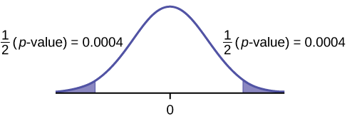
f. \(p\text{-value} = 0.00086\)

g. Reject the \(H_{0}\).
h. At the 5% significance level, from the sample data, there is sufficient evidence to conclude that there is a difference between the proportion of forcible rapes in 2011 and 2010.
Confidence Intervals for the Difference Between Two Independent Population Proportions
If the interest is to estimate how much larger one population proportion is than another population proportion, then a confidence interval rather than a hypothesis test is used. The center of the confidence interval will be the difference between the sample proportions and the margin of error will be the product of the corresponding value of z and the standard error. Putting this together gives the following formula.
Confidence Interval for the Difference Formula \(\PageIndex{6}\)
\(\hat{p}_A - \hat{p}_B \pm z_{\frac{\alpha}{2}}\sqrt{\frac{\hat{p}_c(1-\hat{p}_c)}{n_A}+\frac{\hat{p}_c(1-\hat{p}_c)}{n_B})}\)
Although one can always theoretically use the formula, in practical applications technology is used. When using the TI84+, for example, the menu item to go to is 2-PropZInt and then enter in the number of successes: \(x_1\) and \(x_2\), the sample sizes: \(n_1\) and \(n_2\) and the confidence level (C-Level), and hit ENTER. The online calculator embedded in this section will also easily find the confidence interval.
Example \(\PageIndex{7}\)
How much more likely are puppies in the animal shelter to be adopted in their first week there compared to older dogs? 278 of the 321 puppies sampled were adopted in the first week and 472 of the 649 older dogs were adopted in the first week.
Answer the following questions:
- Is this a confidence interval for the difference of two means or two proportions?
- Which distribution do you use to perform the test?
- What is the random variable?
- What is the lower bound for the 95% confidence interval for the difference?
- What is the upper bound for the 95% confidence interval for the difference?
- State and interpret the 95% confidence interval.
- Interpret the lower bound for the 95% confidence interval.
- Interpret the upper bound for the 95% confidence interval.
- Explain what it means to be 95% confident in the context of the study.
Answer
- two proportions
- \(z\)
- \( \hat{p}_{A} - \hat{p}_{B}\)
- 0.0828
- 0.1948
- The 95% confidence interval is [0.0828, 0.1948]. With 95% confidence, puppies are between 8% and 19% more likely than older dogs to be adopted in their first week at the shelter. This refers to the population of all puppies and older dogs that come into the shelter.
- With 95% confidence, we can state that puppies are at least 8% more likely to be adopted compared to older dogs.
- With 95% confidence, we can state that puppies are no more than 19% more likely to be adopted compared to older dogs.
- If many samples of 321 puppies and 649 older dogs at shelters were looked at, then a different confidence interval would result from each of these samples. 95% of these confidence intervals will contain the true difference between the population proportion of adoptions within the first week and 5% of these confidence intervals will fail to contain the true difference between the population proportion of adoptions within the first week.
Exercise \(\PageIndex{8}\)
How much more likely are women than men over 65 to develop Alzheimer's? 96 of the 893 men over 65 years old observed developed Alzheimer's and 238 of the 1129 women over 65 years old observed developed Alzheimer's. Come up with and interpret the 95% confidence interval for the difference.
Answer
The 95% confidence interval is [-0.1359, -0.0707]. With 95% confidence it can be concluded that for the population of all men and women over 65 years old, that men are between 7% and 14% less likely than women to develop Alzheimer's.
References
- Data from Educational Resources, December catalog.
- Data from Hilton Hotels. Available online at http://www.hilton.com (accessed June 17, 2013).
- Data from Hyatt Hotels. Available online at http://hyatt.com (accessed June 17, 2013).
- Data from Statistics, United States Department of Health and Human Services.
- Data from Whitney Exhibit on loan to San Jose Museum of Art.
- Data from the American Cancer Society. Available online at http://www.cancer.org/index (accessed June 17, 2013).
- Data from the Chancellor’s Office, California Community Colleges, November 1994.
- “State of the States.” Gallup, 2013. Available online at http://www.gallup.com/poll/125066/St...ef=interactive (accessed June 17, 2013).
- “West Nile Virus.” Centers for Disease Control and Prevention. Available online at http://www.cdc.gov/ncidod/dvbid/westnile/index.htm (accessed June 17, 2013).
Chapter Review
- Test of two population proportions from independent samples.
- Random variable: \(\hat{p}_{A} - \hat{p}_{B} =\) difference between the two estimated proportions
- Distribution: normal distribution
Formula Review
Pooled Proportion:
\[p_{c} = \dfrac{x_{A} + x_{B}}{n_{A} + n_{B}}\]
Distribution for the differences:
\[ \hat{p}_{A} - \hat{p}_{B} \sim N\left[0, \sqrt{p_{c}(1-p_{c})\left(\dfrac{1}{n_{A}} + \dfrac{1}{n_{B}}\right)}\right]\]
where the null hypothesis is \(H_{0}: p_{A} = p_{B}\) or \(H_{0}: p_{A} - p_{B} = 0\).
Test Statistic (z-score):
\[z = \dfrac{( \hat{p}_{A} - \hat{p}_{B})}{\sqrt{p_{c}(1-p_{c})\left(\dfrac{1}{n_{A}} + \dfrac{1}{n_{B}}\right)}}\]
where the null hypothesis is \(H_{0}: p_{A} = p_{B}\) or \(H_{0}: p_{A} - p_{B} = 0\).
and
- \( \hat{p}_{A}\) and \( \hat{p}_{B}\) are the sample proportions, \(p_{A}\) and \(p_{B}\) are the population proportions,
- \(P_{c}\) is the pooled proportion, and \(n_{A}\) and \(n_{B}\) are the sample sizes.
Glossary
- Pooled Proportion
- estimate of the common value of \(p_{1}\) and \(p_{2}\).
Contributors and Attributions
Barbara Illowsky and Susan Dean (De Anza College) with many other contributing authors. Content produced by OpenStax College is licensed under a Creative Commons Attribution License 4.0 license. Download for free at http://cnx.org/contents/30189442-699...b91b9de@18.114.


