
7.3: The Central Limit Theorem for Sums
- Page ID
- 20389

\( \newcommand{\vecs}[1]{\overset { \scriptstyle \rightharpoonup} {\mathbf{#1}} } \)
\( \newcommand{\vecd}[1]{\overset{-\!-\!\rightharpoonup}{\vphantom{a}\smash {#1}}} \)
\( \newcommand{\id}{\mathrm{id}}\) \( \newcommand{\Span}{\mathrm{span}}\)
( \newcommand{\kernel}{\mathrm{null}\,}\) \( \newcommand{\range}{\mathrm{range}\,}\)
\( \newcommand{\RealPart}{\mathrm{Re}}\) \( \newcommand{\ImaginaryPart}{\mathrm{Im}}\)
\( \newcommand{\Argument}{\mathrm{Arg}}\) \( \newcommand{\norm}[1]{\| #1 \|}\)
\( \newcommand{\inner}[2]{\langle #1, #2 \rangle}\)
\( \newcommand{\Span}{\mathrm{span}}\)
\( \newcommand{\id}{\mathrm{id}}\)
\( \newcommand{\Span}{\mathrm{span}}\)
\( \newcommand{\kernel}{\mathrm{null}\,}\)
\( \newcommand{\range}{\mathrm{range}\,}\)
\( \newcommand{\RealPart}{\mathrm{Re}}\)
\( \newcommand{\ImaginaryPart}{\mathrm{Im}}\)
\( \newcommand{\Argument}{\mathrm{Arg}}\)
\( \newcommand{\norm}[1]{\| #1 \|}\)
\( \newcommand{\inner}[2]{\langle #1, #2 \rangle}\)
\( \newcommand{\Span}{\mathrm{span}}\) \( \newcommand{\AA}{\unicode[.8,0]{x212B}}\)
\( \newcommand{\vectorA}[1]{\vec{#1}} % arrow\)
\( \newcommand{\vectorAt}[1]{\vec{\text{#1}}} % arrow\)
\( \newcommand{\vectorB}[1]{\overset { \scriptstyle \rightharpoonup} {\mathbf{#1}} } \)
\( \newcommand{\vectorC}[1]{\textbf{#1}} \)
\( \newcommand{\vectorD}[1]{\overrightarrow{#1}} \)
\( \newcommand{\vectorDt}[1]{\overrightarrow{\text{#1}}} \)
\( \newcommand{\vectE}[1]{\overset{-\!-\!\rightharpoonup}{\vphantom{a}\smash{\mathbf {#1}}}} \)
\( \newcommand{\vecs}[1]{\overset { \scriptstyle \rightharpoonup} {\mathbf{#1}} } \)
\( \newcommand{\vecd}[1]{\overset{-\!-\!\rightharpoonup}{\vphantom{a}\smash {#1}}} \)
\(\newcommand{\avec}{\mathbf a}\) \(\newcommand{\bvec}{\mathbf b}\) \(\newcommand{\cvec}{\mathbf c}\) \(\newcommand{\dvec}{\mathbf d}\) \(\newcommand{\dtil}{\widetilde{\mathbf d}}\) \(\newcommand{\evec}{\mathbf e}\) \(\newcommand{\fvec}{\mathbf f}\) \(\newcommand{\nvec}{\mathbf n}\) \(\newcommand{\pvec}{\mathbf p}\) \(\newcommand{\qvec}{\mathbf q}\) \(\newcommand{\svec}{\mathbf s}\) \(\newcommand{\tvec}{\mathbf t}\) \(\newcommand{\uvec}{\mathbf u}\) \(\newcommand{\vvec}{\mathbf v}\) \(\newcommand{\wvec}{\mathbf w}\) \(\newcommand{\xvec}{\mathbf x}\) \(\newcommand{\yvec}{\mathbf y}\) \(\newcommand{\zvec}{\mathbf z}\) \(\newcommand{\rvec}{\mathbf r}\) \(\newcommand{\mvec}{\mathbf m}\) \(\newcommand{\zerovec}{\mathbf 0}\) \(\newcommand{\onevec}{\mathbf 1}\) \(\newcommand{\real}{\mathbb R}\) \(\newcommand{\twovec}[2]{\left[\begin{array}{r}#1 \\ #2 \end{array}\right]}\) \(\newcommand{\ctwovec}[2]{\left[\begin{array}{c}#1 \\ #2 \end{array}\right]}\) \(\newcommand{\threevec}[3]{\left[\begin{array}{r}#1 \\ #2 \\ #3 \end{array}\right]}\) \(\newcommand{\cthreevec}[3]{\left[\begin{array}{c}#1 \\ #2 \\ #3 \end{array}\right]}\) \(\newcommand{\fourvec}[4]{\left[\begin{array}{r}#1 \\ #2 \\ #3 \\ #4 \end{array}\right]}\) \(\newcommand{\cfourvec}[4]{\left[\begin{array}{c}#1 \\ #2 \\ #3 \\ #4 \end{array}\right]}\) \(\newcommand{\fivevec}[5]{\left[\begin{array}{r}#1 \\ #2 \\ #3 \\ #4 \\ #5 \\ \end{array}\right]}\) \(\newcommand{\cfivevec}[5]{\left[\begin{array}{c}#1 \\ #2 \\ #3 \\ #4 \\ #5 \\ \end{array}\right]}\) \(\newcommand{\mattwo}[4]{\left[\begin{array}{rr}#1 \amp #2 \\ #3 \amp #4 \\ \end{array}\right]}\) \(\newcommand{\laspan}[1]{\text{Span}\{#1\}}\) \(\newcommand{\bcal}{\cal B}\) \(\newcommand{\ccal}{\cal C}\) \(\newcommand{\scal}{\cal S}\) \(\newcommand{\wcal}{\cal W}\) \(\newcommand{\ecal}{\cal E}\) \(\newcommand{\coords}[2]{\left\{#1\right\}_{#2}}\) \(\newcommand{\gray}[1]{\color{gray}{#1}}\) \(\newcommand{\lgray}[1]{\color{lightgray}{#1}}\) \(\newcommand{\rank}{\operatorname{rank}}\) \(\newcommand{\row}{\text{Row}}\) \(\newcommand{\col}{\text{Col}}\) \(\renewcommand{\row}{\text{Row}}\) \(\newcommand{\nul}{\text{Nul}}\) \(\newcommand{\var}{\text{Var}}\) \(\newcommand{\corr}{\text{corr}}\) \(\newcommand{\len}[1]{\left|#1\right|}\) \(\newcommand{\bbar}{\overline{\bvec}}\) \(\newcommand{\bhat}{\widehat{\bvec}}\) \(\newcommand{\bperp}{\bvec^\perp}\) \(\newcommand{\xhat}{\widehat{\xvec}}\) \(\newcommand{\vhat}{\widehat{\vvec}}\) \(\newcommand{\uhat}{\widehat{\uvec}}\) \(\newcommand{\what}{\widehat{\wvec}}\) \(\newcommand{\Sighat}{\widehat{\Sigma}}\) \(\newcommand{\lt}{<}\) \(\newcommand{\gt}{>}\) \(\newcommand{\amp}{&}\) \(\definecolor{fillinmathshade}{gray}{0.9}\)Suppose \(X\) is a random variable with a distribution that may be known or unknown (it can be any distribution) and suppose:
- \(\mu_{x}\) = the mean of \(X\)
- \(\sigma_{x}\) = the standard deviation of \(X\)
If you draw random samples of size \(n\), then as \(n\) increases, the random variable \(\sum X\) consisting of sums tends to be normally distributed and
\[\sum X \sim N((n)(\mu_{x}), (\sqrt{n})(\sigma_{x})).\]
The central limit theorem for sums says that if you keep drawing larger and larger samples and taking their sums, the sums form their own normal distribution (the sampling distribution), which approaches a normal distribution as the sample size increases. The normal distribution has a mean equal to the original mean multiplied by the sample size and a standard deviation equal to the original standard deviation multiplied by the square root of the sample size.
The random variable \(\sum X\) has the following z-score associated with it:
- \(\sum x\) is one sum.
- \(z = \frac{\sum x - (n)(\mu_{x})}{(\sqrt{n})(\sigma_{x})}\)
- \((n)(\mu_{x})\)= the mean of \(\sum X\)
- \((\sqrt{n})(\sigma_{x})\)= standard deviation of \(\sum X\)
Online Calculator for sums
| Low: | High: | Mean: | Std. Dev.: | n= | p= |
Enter the Low, High, Mean, Standard Deviation (ST. Dev.), Sample Size (n), and then hit Calculate to find the probability. You can also enter in the probability and leave either the Low or the High blank, and it will find the missing bound.
Example \(\PageIndex{1}\)
An unknown distribution has a mean of 90 and a standard deviation of 15. A sample of size 80 is drawn randomly from the population.
- Find the probability that the sum of the 80 values (or the total of the 80 values) is more than 7,500.
- Find the sum that is 1.5 standard deviations above the mean of the sums.
Answer
Let \(X =\) one value from the original unknown population. The probability question asks you to find a probability for the sum (or total of) 80 values.
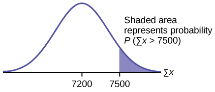
\(\sum X =\) the sum or total of 80 values. Since \(\mu_{x} = 90\), \(\sigma_{x} = 15\), and \(n = 80\), \(\sum X \sim N((80)(90),(\sqrt{80})(15))\)
- mean of the sums \(= (n)(\mu_{x}) = (80)(90) = 7,200\)
- standard deviation of the sums \(= (\sqrt{n})(\sigma_{x}) = (\sqrt{80})(15) = (80)(15)\)
- sum of 80 values \(= \sum X = 7,500\)
a. Find \(P(\sum X > 7,500)\)
\(P(\sum X > 7,500) = 0.0127\)
Low = 7500, High = 999999, Mean = (80)(90) = 7200, St. Dev. = \( (\sqrt{80})(15) = 0.0127\), p =
\(P(\sum x > 7500) = 0.0127 \)
b. Find \(\sum x\) where \(z = 1.5\).
\(\sum x = (n)(\nu_{x}) + (z)(\sqrt{n})(\sigma_{x}) = (80)(90) + (1.5)(\sqrt{80})(15) = 7,401.2\)
Exercise \(\PageIndex{1}\)
An unknown distribution has a mean of 45 and a standard deviation of eight. A sample size of 50 is drawn randomly from the population. Find the probability that the sum of the 50 values is more than 2,400.
Answer
0.0040
Exercise \(\PageIndex{2}\)
In a study reported Oct. 29, 2012 on the Flurry Blog, the mean age of tablet users is 35 years. Suppose the standard deviation is ten years. The sample size is 39.
- What are the mean and standard deviation for the sum of the ages of tablet users? What is the distribution?
- Find the probability that the sum of the ages is between 1,400 and 1,500 years.
- Find the 90th percentile for the sum of the 39 ages.
Answer
- \(\mu_{\sum X} = n\mu_{X} = 1,365\) and \(\sigma_{\sum X} = \sqrt{n}\sigma_{x} = 62.4\)
The distribution is normal for sums by the central limit theorem. - Low = 1400, High = 1500, Mean = (39)(35) = 1365, St. Dev. = \( (\sqrt{39})(10) = 62.4\), p =
\(P(1400 < \sum_{X} < 1500) = 0.2723\) - Let \(k\) = the 90th percentile.
Low = -999999, High = , Mean = 1365, St. Dev. = 62.4, p = 0.90
\(k = 1445.0\)
Example \(\PageIndex{2}\)
The mean number of minutes for app engagement by a tablet user is 8.2 minutes. Suppose the standard deviation is one minute. Take a sample of size 70.
- What are the mean and standard deviation for the sums?
- Find the 95th percentile for the sum of the sample. Interpret this value in a complete sentence.
- Find the probability that the sum of the sample is at least ten hours.
Answer
- \(\mu_{\sum X} = n\mu_{X}= 70(8.2) = 574\) minutes and \(\sigma_{\sum X} (\sqrt{n})(\sigma_{x}) = (\sqrt{70})(1) = 8.37\) minutes
- Let \(k\) = the 95th percentile.
Low = -99999, High = , Mean = 574, St. Dev. = 8.37, p = 0.95
\(k = 587.76\) minutes
Ninety five percent of the app engagement times are at most 587.76 minutes. - Ten hours = 600 minutes
Low = 600, High = 99999 , Mean = 574, St. Dev. = 8.37, p =
\(P(\sum X \geq 600) = 0.0009\)
Exercise \(\PageIndex{3}\)
The mean number of minutes for app engagement by a table use is 8.2 minutes. Suppose the standard deviation is one minute. Take a sample size of 70.
- What is the probability that the sum of the sample is between seven hours and ten hours? What does this mean in context of the problem?
- Find the 84th and 16th percentiles for the sum of the sample. Interpret these values in context.
Answer
- 7 hours = 420 minutes
10 hours = 600 minutes
Low = 420, High = 600 , Mean = 574, St. Dev. = 8.37, p =
\( P(420 \leq \sum X \leq 600) = 0.9991\)
This means that for this sample sums there is a 99.9% chance that the sums of usage minutes will be between 420 minutes and 600 minutes. - Low = -99999, High = , Mean = 574, St. Dev. = 8.37, p = 0.84
The 16th percentile is 582.32.
Low = -99999, High = , Mean = 574, St. Dev. = 8.37, p = 0.16
The 16th percentile is 565.68.
Since 84% of the app engagement times are at most 582.32 minutes and 16% of the app engagement times are at most 565.68 minutes, we may state that 68% of the app engagement times are between 565.68 minutes and 582.32 minutes.
References
- Farago, Peter. “The Truth About Cats and Dogs: Smartphone vs Tablet Usage Differences.” The Flurry Blog, 2013. Posted October 29, 2012. Available online at http://blog.flurry.com (accessed May 17, 2013).
Chapter Review
The central limit theorem tells us that for a population with any distribution, the distribution of the sums for the sample means approaches a normal distribution as the sample size increases. In other words, if the sample size is large enough, the distribution of the sums can be approximated by a normal distribution even if the original population is not normally distributed. Additionally, if the original population has a mean of \(\mu_{x}\) and a standard deviation of \(\sigma_{x}\), the mean of the sums is \(n\)\(\mu_{x}\) and the standard deviation is (\(\sqrt{n}\))(\(\sigma_{x}\)) where \(n\) is the sample size.
Formula Review
- The Central Limit Theorem for Sums: \(\sum X ~ N[(n)(\mu_{x}, (\sqrt{n})(\sigma_{x}))]\)
- Mean for Sums \((\sum X): (n)(\mu_{x})\)
- The Central Limit Theorem for Sums \(z\)-score and standard deviation for sums: \(z \text{ for the sample mean} = \frac{\sum x - (n)(\mu_{x})}{(\sqrt{n})(\sigma_{x})}\)
- Standard deviation for Sums \((\sum X): (\sqrt{n})(\sigma_{x})\)