10.3: Inference for Regression and Correlation
- Page ID
- 16375
\( \newcommand{\vecs}[1]{\overset { \scriptstyle \rightharpoonup} {\mathbf{#1}} } \)
\( \newcommand{\vecd}[1]{\overset{-\!-\!\rightharpoonup}{\vphantom{a}\smash {#1}}} \)
\( \newcommand{\dsum}{\displaystyle\sum\limits} \)
\( \newcommand{\dint}{\displaystyle\int\limits} \)
\( \newcommand{\dlim}{\displaystyle\lim\limits} \)
\( \newcommand{\id}{\mathrm{id}}\) \( \newcommand{\Span}{\mathrm{span}}\)
( \newcommand{\kernel}{\mathrm{null}\,}\) \( \newcommand{\range}{\mathrm{range}\,}\)
\( \newcommand{\RealPart}{\mathrm{Re}}\) \( \newcommand{\ImaginaryPart}{\mathrm{Im}}\)
\( \newcommand{\Argument}{\mathrm{Arg}}\) \( \newcommand{\norm}[1]{\| #1 \|}\)
\( \newcommand{\inner}[2]{\langle #1, #2 \rangle}\)
\( \newcommand{\Span}{\mathrm{span}}\)
\( \newcommand{\id}{\mathrm{id}}\)
\( \newcommand{\Span}{\mathrm{span}}\)
\( \newcommand{\kernel}{\mathrm{null}\,}\)
\( \newcommand{\range}{\mathrm{range}\,}\)
\( \newcommand{\RealPart}{\mathrm{Re}}\)
\( \newcommand{\ImaginaryPart}{\mathrm{Im}}\)
\( \newcommand{\Argument}{\mathrm{Arg}}\)
\( \newcommand{\norm}[1]{\| #1 \|}\)
\( \newcommand{\inner}[2]{\langle #1, #2 \rangle}\)
\( \newcommand{\Span}{\mathrm{span}}\) \( \newcommand{\AA}{\unicode[.8,0]{x212B}}\)
\( \newcommand{\vectorA}[1]{\vec{#1}} % arrow\)
\( \newcommand{\vectorAt}[1]{\vec{\text{#1}}} % arrow\)
\( \newcommand{\vectorB}[1]{\overset { \scriptstyle \rightharpoonup} {\mathbf{#1}} } \)
\( \newcommand{\vectorC}[1]{\textbf{#1}} \)
\( \newcommand{\vectorD}[1]{\overrightarrow{#1}} \)
\( \newcommand{\vectorDt}[1]{\overrightarrow{\text{#1}}} \)
\( \newcommand{\vectE}[1]{\overset{-\!-\!\rightharpoonup}{\vphantom{a}\smash{\mathbf {#1}}}} \)
\( \newcommand{\vecs}[1]{\overset { \scriptstyle \rightharpoonup} {\mathbf{#1}} } \)
\(\newcommand{\longvect}{\overrightarrow}\)
\( \newcommand{\vecd}[1]{\overset{-\!-\!\rightharpoonup}{\vphantom{a}\smash {#1}}} \)
\(\newcommand{\avec}{\mathbf a}\) \(\newcommand{\bvec}{\mathbf b}\) \(\newcommand{\cvec}{\mathbf c}\) \(\newcommand{\dvec}{\mathbf d}\) \(\newcommand{\dtil}{\widetilde{\mathbf d}}\) \(\newcommand{\evec}{\mathbf e}\) \(\newcommand{\fvec}{\mathbf f}\) \(\newcommand{\nvec}{\mathbf n}\) \(\newcommand{\pvec}{\mathbf p}\) \(\newcommand{\qvec}{\mathbf q}\) \(\newcommand{\svec}{\mathbf s}\) \(\newcommand{\tvec}{\mathbf t}\) \(\newcommand{\uvec}{\mathbf u}\) \(\newcommand{\vvec}{\mathbf v}\) \(\newcommand{\wvec}{\mathbf w}\) \(\newcommand{\xvec}{\mathbf x}\) \(\newcommand{\yvec}{\mathbf y}\) \(\newcommand{\zvec}{\mathbf z}\) \(\newcommand{\rvec}{\mathbf r}\) \(\newcommand{\mvec}{\mathbf m}\) \(\newcommand{\zerovec}{\mathbf 0}\) \(\newcommand{\onevec}{\mathbf 1}\) \(\newcommand{\real}{\mathbb R}\) \(\newcommand{\twovec}[2]{\left[\begin{array}{r}#1 \\ #2 \end{array}\right]}\) \(\newcommand{\ctwovec}[2]{\left[\begin{array}{c}#1 \\ #2 \end{array}\right]}\) \(\newcommand{\threevec}[3]{\left[\begin{array}{r}#1 \\ #2 \\ #3 \end{array}\right]}\) \(\newcommand{\cthreevec}[3]{\left[\begin{array}{c}#1 \\ #2 \\ #3 \end{array}\right]}\) \(\newcommand{\fourvec}[4]{\left[\begin{array}{r}#1 \\ #2 \\ #3 \\ #4 \end{array}\right]}\) \(\newcommand{\cfourvec}[4]{\left[\begin{array}{c}#1 \\ #2 \\ #3 \\ #4 \end{array}\right]}\) \(\newcommand{\fivevec}[5]{\left[\begin{array}{r}#1 \\ #2 \\ #3 \\ #4 \\ #5 \\ \end{array}\right]}\) \(\newcommand{\cfivevec}[5]{\left[\begin{array}{c}#1 \\ #2 \\ #3 \\ #4 \\ #5 \\ \end{array}\right]}\) \(\newcommand{\mattwo}[4]{\left[\begin{array}{rr}#1 \amp #2 \\ #3 \amp #4 \\ \end{array}\right]}\) \(\newcommand{\laspan}[1]{\text{Span}\{#1\}}\) \(\newcommand{\bcal}{\cal B}\) \(\newcommand{\ccal}{\cal C}\) \(\newcommand{\scal}{\cal S}\) \(\newcommand{\wcal}{\cal W}\) \(\newcommand{\ecal}{\cal E}\) \(\newcommand{\coords}[2]{\left\{#1\right\}_{#2}}\) \(\newcommand{\gray}[1]{\color{gray}{#1}}\) \(\newcommand{\lgray}[1]{\color{lightgray}{#1}}\) \(\newcommand{\rank}{\operatorname{rank}}\) \(\newcommand{\row}{\text{Row}}\) \(\newcommand{\col}{\text{Col}}\) \(\renewcommand{\row}{\text{Row}}\) \(\newcommand{\nul}{\text{Nul}}\) \(\newcommand{\var}{\text{Var}}\) \(\newcommand{\corr}{\text{corr}}\) \(\newcommand{\len}[1]{\left|#1\right|}\) \(\newcommand{\bbar}{\overline{\bvec}}\) \(\newcommand{\bhat}{\widehat{\bvec}}\) \(\newcommand{\bperp}{\bvec^\perp}\) \(\newcommand{\xhat}{\widehat{\xvec}}\) \(\newcommand{\vhat}{\widehat{\vvec}}\) \(\newcommand{\uhat}{\widehat{\uvec}}\) \(\newcommand{\what}{\widehat{\wvec}}\) \(\newcommand{\Sighat}{\widehat{\Sigma}}\) \(\newcommand{\lt}{<}\) \(\newcommand{\gt}{>}\) \(\newcommand{\amp}{&}\) \(\definecolor{fillinmathshade}{gray}{0.9}\)How do you really say you have a correlation? Can you test to see if there really is a correlation? Of course, the answer is yes. The hypothesis test for correlation is as follows:
Hypothesis Test for Correlation:
- State the random variables in words.
x = independent variable
y = dependent variable - State the null and alternative hypotheses and the level of significance
\(\begin{array}{l}{H_{o} : \rho=0 \text { (There is no correlation) }} \\ {H_{A} : \rho \neq 0 \text { (There is a correlation) }} \\ {\text { or }} \\ {H_{A} : \rho<0 \text { (There is a negative correlation) }} \\ {\text { or }} \\ {H_{A} : \rho>0 \text { (There is a postive correlation) }}\end{array}\)
Also, state your \(\alpha\) level here. - State and check the assumptions for the hypothesis test
The assumptions for the hypothesis test are the same assumptions for regression and correlation. - Find the test statistic and p-value
\(t=\dfrac{r}{\sqrt{\dfrac{1-r^{2}}{n-2}}}\)
with degrees of freedom = df = n - 2
p-value: Using the TI-83/84: tcdf(lower limit, upper limit, df)Note
If \(H_{A} : \rho<0\), then lower limit is -1E99 and upper limit is your test statistic. If \(H_{A} : \rho>0\), then lower limit is your test statistic and the upper limit is 1E99. If \(H_{A} : \rho \neq 0\), then find the p-value for \(H_{A} : \rho<0\), and multiply by 2.
Using R: pt(t, df)
Note
If \(H_{A} : \rho<0\), then use pt(t, df), If \(H_{A} : \rho>0\), then use \(1-\mathrm{pt}(t, d f)\). If \(H_{A} : \rho \neq 0\), then find the p-value for \(H_{A} : \rho<0\), and multiply by 2.
- Conclusion
This is where you write reject \(H_{o}\) or fail to reject \(H_{o}\). The rule is: if the p-value < \(\alpha\), then reject \(H_{o}\). If the p-value \(\geq \alpha\), then fail to reject \(H_{o}\). - Interpretation
This is where you interpret in real world terms the conclusion to the test. The conclusion for a hypothesis test is that you either have enough evidence to show \(H_{A}\) is true, or you do not have enough evidence to show \(H_{A}\) is true.
Note
The TI-83/84 calculator results give you the test statistic and the p-value. In R, the command for getting the test statistic and p-value is cor.test(independent variable, dependent variable, alternative = "less" or "greater"). Use less for \(H_{A} : \rho<0\), use greater for \(H_{A} : \rho>0\), and leave off this command for \(H_{A} : \rho \neq 0\).
Example \(\PageIndex{1}\) Testing the claim of a linear correlation
Is there a positive correlation between beer’s alcohol content and calories? To determine if there is a positive linear correlation, a random sample was taken of beer’s alcohol content and calories for several different beers ("Calories in beer," 2011), and the data is in Example \(\PageIndex{1}\). Test at the 5% level.
Solution
- State the random variables in words.
x = alcohol content in the beer
y = calories in 12 ounce beer - State the null and alternative hypotheses and the level of significance.
Since you are asked if there is a positive correlation, \(\rho> 0\).
\(\begin{array}{l}{H_{o} : \rho=0} \\ {H_{A} : \rho>0} \\ {\alpha=0.05}\end{array}\) - State and check the assumptions for the hypothesis test.
The assumptions for the hypothesis test were already checked in Example \(\PageIndex{2}\). - Find the test statistic and p-value.
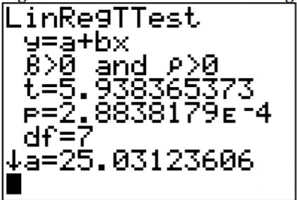
The results from the TI-83/84 calculator are in Figure \(\PageIndex{1}\).
.png?revision=1)
Figure \(\PageIndex{1}\): Results for Linear Regression Test on TI-83/84
Test statistic: t \(\approx\) 5.938 and p-value: \(p \approx 2.884 \times 10^{-4}\)
If we ran the same test using the software package R we would get
Pearson's product-moment correlation
data: alcohol and calories
t = 5.9384, df = 7, p-value = 0.0002884
alternative hypothesis: true correlation is greater than 0
95 percent confidence interval:
0.7046161 1.0000000
sample estimates:
cor
0.9134414
Test statistic: t \(\approx\) 5.9384 and p-value: \(p \approx 0.0002884\) - Conclusion
Reject \(H_{o}\) since the p-value is less than 0.05. - Interpretation
There is enough evidence to show that there is a positive correlation between alcohol content and number of calories in a 12-ounce bottle of beer.
Prediction Interval
Using the regression equation you can predict the number of calories from the alcohol content. However, you only find one value. The problem is that beers vary a bit in calories even if they have the same alcohol content. It would be nice to have a range instead of a single value. The range is called a prediction interval. To find this, you need to figure out how much error is in the estimate from the regression equation. This is known as the standard error of the estimate.
Definition
Standard Error of the Estimate
This is the sum of squares of the residuals
\(s_{e}=\sqrt{\dfrac{\sum(y-\hat{y})^{2}}{n-2}}\)
This formula is hard to work with, so there is an easier formula. You can also find the value from technology, such as the calculator.
\(s_{e}=\sqrt{\dfrac{S S_{y}-b^{*} S S_{x y}}{n-2}}\)
Example \(\PageIndex{2}\) finding the standard error of the estimate
Find the standard error of the estimate for the beer data. To determine if there is a positive linear correlation, a random sample was taken of beer’s alcohol content and calories for several different beers ("Calories in beer," 2011), and the data are in Example \(\PageIndex{1}\).
Solution
x = alcohol content in the beer
y = calories in 12 ounce beer
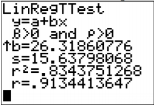
Using the TI-83/84, the results are in Figure \(\PageIndex{2}\).
.png?revision=1)
The s in the results is the standard error of the estimate. So \(s_{e} \approx 15.64\). From this output, you can also see that the slope is 26.319.
If you want to know how to calculate the standard error of the estimate from the formula, refer to Example \(\PageIndex{3}\).
Example \(\PageIndex{3}\) finding the standard error of the estimate from the formula
Find the standard error of the estimate for the beer data using the formula. To determine if there is a positive linear correlation, a random sample was taken of beer’s alcohol content and calories for several different beers ("Calories in beer," 2011), and the data are in Example \(\PageIndex{1}\).
Solution
x = alcohol content in the beer
y = calories in 12 ounce beer
From Example \(\PageIndex{3}\) :
\(\begin{array}{l}{S S_{y}=\sum(y-\overline{y})^{2}=10335.56} \\ {S S_{x y}=\sum(x-\overline{x})(y-\overline{y})=327.6666} \\ {n=9} \\ {b=26.3}\end{array}\)
The standard error of the estimate is
\(\begin{aligned} s_{e} &=\sqrt{\dfrac{S S_{y}-b^{*} S S_{x y}}{n-2}} \\ &=\sqrt{\dfrac{10335.56-26.3(327.6666)}{9-2}} \\ &=15.67 \end{aligned}\)
Prediction Interval for an Individual y
Given the fixed value \(x_{0}\), the prediction interval for an individual y is
\(\hat{y}-E<y<\hat{y}+E\)
where
\(\begin{array}{l}{\hat{y}=a+b x} \\ {E=t_{c} s_{e} \sqrt{1+\dfrac{1}{n}+\dfrac{\left(x_{o}-\overline{x}\right)^{2}}{S S_{x}}}} \\ {d f=n-2}\end{array}\)
Note
To find \(S S_{x}=\sum(x-\overline{x})^{2}\) remember, the standard derivation formula from chapter 3 \(s_{x}=\sqrt{\dfrac{\sum(x-\overline{x})^{2}}{n-1}}\)
So, \(s_{x}=\sqrt{\dfrac{S S_{x}}{n-1}}\)
Now solve for \(S S_{x}\)
\(S S_{x}=s_{x}^{2}(n-1)\)
You can get the standard deviation from technology.
R will produce the prediction interval for you. The commands are (Note you probably already did the lm.out command. You do not need to do it again.)
lm.out = lm(dependent variable ~ independent variable) – calculates the linear model
predict(lm.out, newdata=list(independent variable = value), interval="prediction", level=C) – will compute a prediction interval for the independent variable set to a particular value (put that value in place of the word value), at a particular C level (given as a decimal)
Example \(\PageIndex{4}\) find the prediction interval
Find a 95% prediction interval for the number of calories when the alcohol content is 6.5% using a random sample taken of beer’s alcohol content and calories ("Calories in beer," 2011). The data are in Example \(\PageIndex{1}\).
Solution
x = alcohol content in the beer
y = calories in 12 ounce beer
Computing the prediction interval using the TI-83/84 calculator:
From Example \(\PageIndex{2}\)
\(\begin{array}{l}{\hat{y}=25.0+26.3 x} \\ {x_{o}=6.50} \\ {\hat{y}=25.0+26.3(6.50)=196 \text { calories }}\end{array}\)
From Example #10.3.2
\(s_{e} \approx 15.64\)
.png?revision=1)
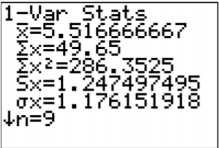
\(\begin{array}{l}{\overline{x}=5.517} \\ {s_{x}=1.247497495} \\ {n=9}\end{array}\)
Now you can find
\(\begin{aligned} S S_{x} &=s_{x}^{2}(n-1) \\ &=(1.247497495)^{2}(9-1) \\ &=12.45 \\ d f &=n-2=9-2=7 \end{aligned}\)
Now look in table A.2. Go down the first column to 7, then over to the column headed with 95%.
\(t_{c}=2.365\)
\(\begin{aligned} E &=t_{c} s_{e} \sqrt{1+\dfrac{1}{n}+\dfrac{\left(x_{o}-\overline{x}\right)^{2}}{S S_{x}}} \\ &=2.365(15.64) \sqrt{1+\dfrac{1}{9}+\dfrac{(6.50-5.517)^{2}}{12.45}} \\ &=40.3 \end{aligned}\)
Prediction interval is
\(\begin{array}{l}{\hat{y}-E<y<\hat{y}+E} \\ {196-40.3<y<196+40.3} \\ {155.7<y<236.3}\end{array}\)
Computing the prediction interval using R:
predict(lm.out, newdata=list(alcohol=6.5), interval = "prediction", level=0.95)
\(\begin{array}{ccc}{}&{\text { fit }} & {\text { lwr }} & {\text { upr }} \\ {1} & {196.1022} & {155.7847}&{236 .4196}\end{array}\)
fit = \(\hat{\mathcal{Y}}\) when x = 6.5%. lwr = lower limit of prediction interval. upr = upper limit of prediction interval. So the prediction interval is \(155.8<y<236.4\).
Statistical interpretation: There is a 95% chance that the interval \(155.8<y<236.4\) contains the true value for the calories when the alcohol content is 6.5%.
Real world interpretation: If a beer has an alcohol content of 6.50% then it has between 156 and 236 calories.
Example \(\PageIndex{5}\) Doing a correlation and regression analysis using the ti-83/84
Example \(\PageIndex{1}\) contains randomly selected high temperatures at various cities on a single day and the elevation of the city.
| Elevation (in feet) | 7000 | 4000 | 6000 | 3000 | 7000 | 4500 | 5000 |
|---|---|---|---|---|---|---|---|
| Temperature (°F) | 50 | 60 | 48 | 70 | 55 | 55 | 60 |
- State the random variables.
- Find a regression equation for elevation and high temperature on a given day.
- Find the residuals and create a residual plot.
- Use the regression equation to estimate the high temperature on that day at an elevation of 5500 ft.
- Use the regression equation to estimate the high temperature on that day at an elevation of 8000 ft.
- Between the answers to parts d and e, which estimate is probably more accurate and why?
- Find the correlation coefficient and coefficient of determination and interpret both.
- Is there enough evidence to show a negative correlation between elevation and high temperature? Test at the 5% level.
- Find the standard error of the estimate.
- Using a 95% prediction interval, find a range for high temperature for an elevation of 6500 feet.
Solution
a. x = elevation
y = high temperature
b.
- A random sample was taken as stated in the problem.
- The distribution for each high temperature value is normally distributed for every value of elevation.
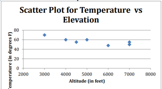
- Look at the scatter plot of high temperature versus elevation.
.png?revision=1)
Figure \(\PageIndex{4}\): Scatter Plot of Temperature Versus Elevation
The scatter plot looks fairly linear. - There are no points that appear to be outliers.
- The residual plot for temperature versus elevation appears to be fairly random. (See Figure \(\PageIndex{7}\).)
It appears that the high temperature is normally distributed.
- Look at the scatter plot of high temperature versus elevation.
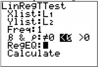
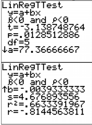
All calculations computed using the TI-83/84 calculator.
.png?revision=1)
.png?revision=1)
\(\hat{y}=77.4-0.0039 x\)
c.
| x | y | \(\hat{\mathcal{Y}}\) | \(y-\hat{y}\) |
|---|---|---|---|
| 7000 | 50 | 50.1 | -0.1 |
| 4000 | 60 | 61.8 | -1.8 |
| 6000 | 48 | 54.0 | -6.0 |
| 3000 | 70 | 65.7 | 4.3 |
| 7000 | 55 | 50.1 | 4.9 |
| 4500 | 55 | 59.85 | -4.85 |
| 5000 | 60 | 57.9 | 2.1 |
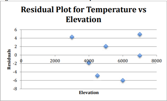.png?revision=1)
The residuals appear to be fairly random.
d.
\(\begin{array}{l}{x_{o}=5500} \\ {\hat{y}=77.4-0.0039(5500)=55.95^{\circ} F}\end{array}\)
e.
\(\begin{array}{l}{x_{o}=8000} \\ {\hat{y}=77.4-0.0039(8000)=46.2^{\circ} F}\end{array}\)
f. Part d is more accurate, since it is interpolation and part e is extrapolation.
g. From Figure \(\PageIndex{6}\), the correlation coefficient is r \(\approx\) -0.814, which is moderate to strong negative correlation.
From Figure \(\PageIndex{6}\), the coefficient of determination is \(r^{2} \approx 0.663\), which means that 66.3% of the variability in high temperature is explained by the linear model. The other 33.7% is explained by other variables such as local weather conditions.
h.
- State the random variables in words.
x = elevation
y = high temperature - State the null and alternative hypotheses and the level of significance
\(\begin{array}{l}{H_{o} : \rho=0} \\ {H_{A} : \rho<0} \\ {\alpha=0.05}\end{array}\) - State and check the assumptions for the hypothesis test The assumptions for the hypothesis test were already checked part b.
- Find the test statistic and p-value
From Figure \(\PageIndex{6}\),
Test statistic:
\(t \approx-3.139\)
p-value:
\(p \approx 0.0129\) - Conclusion
Reject \(H_{o}\) since the p-value is less than 0.05. - Interpretation
There is enough evidence to show that there is a negative correlation between elevation and high temperatures.
i. From Figure \(\PageIndex{6}\),
\(s_{e} \approx 4.677\)
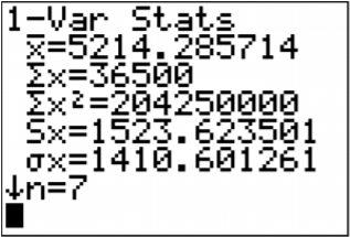
j. \(\hat{y}=77.4-0.0039(6500) \approx 52.1^{\circ} F\)
.png?revision=1)
\(\begin{array}{l}{\overline{x}=5214.29} \\ {s_{x}=1523.624} \\ {n=7}\end{array}\)
Now you can find
\(\begin{aligned} S S_{x} &=s_{x}^{2}(n-1) \\ &=(1523.623501)^{2}(7-1) \\ &=13928571.43 \\ d f &=n-2=7-2=5 \end{aligned}\)
Now look in table A.2. Go down the first column to 5, then over to the column headed with 95%.
\(t_{c}=2.571\)
So
\(\begin{aligned} E &=t_{c} s_{e} \sqrt{1+\dfrac{1}{n}+\dfrac{\left(x_{o}-\overline{x}\right)^{2}}{S S_{x}}} \\ &=2.571(4.677) \sqrt{1+\dfrac{1}{7}+\dfrac{(6500-5214.29)^{2}}{13928571.43}} \\ &=13.5 \end{aligned}\)
Prediction interval is
\(\begin{array}{l}{\hat{y}-E<y<\hat{y}+E} \\ {52.1-13.5<y<52.1+13.5} \\ {38.6<y<65.6}\end{array}\)
Statistical interpretation: There is a 95% chance that the interval \(38.6<y<65.6\) contains the true value for the temperature at an elevation of 6500 feet.
Real world interpretation: A city of 6500 feet will have a high temperature between 38.6°F and 65.6°F. Though this interval is fairly wide, at least the interval tells you that the temperature isn’t that warm.
Example \(\PageIndex{6}\) doing a correlation and regression analysis using r
Example \(\PageIndex{1}\) contains randomly selected high temperatures at various cities on a single day and the elevation of the city.
- State the random variables.
- Find a regression equation for elevation and high temperature on a given day.
- Find the residuals and create a residual plot.
- Use the regression equation to estimate the high temperature on that day at an elevation of 5500 ft.
- Use the regression equation to estimate the high temperature on that day at an elevation of 8000 ft.
- Between the answers to parts d and e, which estimate is probably more accurate and why?
- Find the correlation coefficient and coefficient of determination and interpret both.
- Is there enough evidence to show a negative correlation between elevation and high temperature? Test at the 5% level.
- Find the standard error of the estimate.
- Using a 95% prediction interval, find a range for high temperature for an elevation of 6500 feet.
Solution
a. x = elevation
y = high temperature
b.
- A random sample was taken as stated in the problem.
- The distribution for each high temperature value is normally distributed for every value of elevation.
- Look at the scatter plot of high temperature versus elevation.
R command: plot(elevation, temperature, main="Scatter Plot for Temperature vs Elevation", xlab="Elevation (feet)", ylab="Temperature (degrees F)", ylim=c(0,80))
.png?revision=1)
Figure \(\PageIndex{9}\): Scatter Plot of Temperature Versus Elevation
The scatter plot looks fairly linear. - The residual plot for temperature versus elevation appears to be fairly random. (See Figure 10.3.10.)
It appears that the high temperature is normally distributed.
- Look at the scatter plot of high temperature versus elevation.
Below is a plot of the residuals.
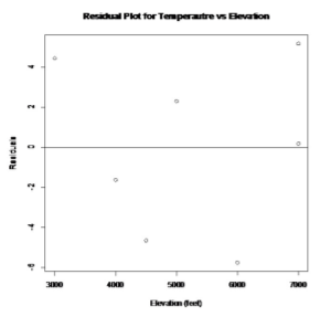.png?revision=1)
The residuals appear to be fairly random.
d. \(\begin{array}{l}{x_{o}=5500} \\ {\hat{y}=77.4-0.0039(5500)=55.95^{\circ} F}\end{array}\)
e. \(\begin{array}{l}{x_{o}=8000} \\ {\hat{y}=77.4-0.0039(8000)=46.2^{\circ} F}\end{array}\)
f. Part d is more accurate, since it is interpolation and part e is extrapolation.
g. \(r \approx-0.814\), which is moderate to strong negative correlation.
So \(r^{2} \approx 0.663\), which means that 66.3% of the variability in high temperature is explained by the linear model. The other 33.7% is explained by other variables such as local weather conditions.
h.
- State the random variables in words.
x = elevation
y = high temperature - . State the null and alternative hypotheses and the level of significance
\(\begin{array}{l}{H_{o} : \rho=0} \\ {H_{A} : \rho<0} \\ {\alpha=0.05}\end{array}\) - State and check the assumptions for the hypothesis test.
The assumptions for the hypothesis test were already checked part b. - Find the test statistic and p-value
t = -3.1387, df = 5, p-value = 0.01285
alternative hypothesis: true correlation is less than 0
95 percent confidence interval:
-1.0000000 -0.3074247
sample estimates:
cor
-0.8144564
Test statistic: \(t \approx-3.1387\) and p-value: \(p \approx 0.01285\) - Conclusion
Reject \(H_{o}\) since the p-value is less than 0.05. - Interpretation
There is enough evidence to show that there is a negative correlation between elevation and high temperatures.
i. From summary(lm.out), Residual standard error: 4.677.
So, \(s_{e} \approx 4.677\)
j. When x = 6500 feet, \(\hat{y}=51.8^{\circ} F \text { and } 38.29672<y<65.30328\).
Statistical interpretation: There is a 95% chance that the interval \(38.3<y<65.3\) contains the true value for the temperature at an elevation of 6500 feet.
Real world interpretation: A city of 6500 feet will have a high temperature between 38.3°F and 65.3°F. Though this interval is fairly wide, at least the interval tells you that the temperature isn’t that warm.
Homework
Exercise \(\PageIndex{1}\)
For each problem, state the random variables. The data sets in this section are in the homework for section 10.1 and were also used in section 10.2. If you removed any data points as outliers in the other sections, remove them in this sections homework too.
- When an anthropologist finds skeletal remains, they need to figure out the height of the person. The height of a person (in cm) and the length of their metacarpal bone one (in cm) were collected and are in Example \(\PageIndex{5}\) ("Prediction of height," 2013).
- Test at the 1% level for a positive correlation between length of metacarpal bone one and height of a person.
- Find the standard error of the estimate.
- Compute a 99% prediction interval for height of a person with a metacarpal length of 44 cm.
- Example \(\PageIndex{6}\) contains the value of the house and the amount of rental income in a year that the house brings in ("Capital and rental," 2013).
- Test at the 5% level for a positive correlation between house value and rental amount.
- Find the standard error of the estimate.
- Compute a 95% prediction interval for the rental income on a house worth $230,000.
- The World Bank collects information on the life expectancy of a person in each country ("Life expectancy at," 2013) and the fertility rate per woman in the country ("Fertility rate," 2013). The data for 24 randomly selected countries for the year 2011 are in Example \(\PageIndex{7}\).
- Test at the 1% level for a negative correlation between fertility rate and life expectancy.
- Find the standard error of the estimate.
- Compute a 99% prediction interval for the life expectancy for a country that has a fertility rate of 2.7.
- The World Bank collected data on the percentage of GDP that a country spends on health expenditures ("Health expenditure," 2013) and also the percentage of women receiving prenatal care ("Pregnant woman receiving," 2013). The data for the countries where this information is available for the year 2011 are in Example \(\PageIndex{8}\).
- Test at the 5% level for a correlation between percentage spent on health expenditure and the percentage of women receiving prenatal care.
- Find the standard error of the estimate.
- Compute a 95% prediction interval for the percentage of woman receiving prenatal care for a country that spends 5.0 % of GDP on health expenditure.
- The height and weight of baseball players are in Example \(\PageIndex{9}\) ("MLB heightsweights," 2013).
- Test at the 5% level for a positive correlation between height and weight of baseball players.
- Find the standard error of the estimate.
- Compute a 95% prediction interval for the weight of a baseball player that is 75 inches tall.
- Different species have different body weights and brain weights are in Example \(\PageIndex{10}\). ("Brain2bodyweight," 2013).
- Test at the 1% level for a positive correlation between body weights and brain weights.
- Find the standard error of the estimate.
- Compute a 99% prediction interval for the brain weight for a species that has a body weight of 62 kg.
- A random sample of beef hotdogs was taken and the amount of sodium (in mg) and calories were measured. ("Data hotdogs," 2013) The data are in Example \(\PageIndex{11}\).
- Test at the 5% level for a correlation between amount of calories and amount of sodium.
- Find the standard error of the estimate.
- Compute a 95% prediction interval for the amount of sodium a beef hotdog has if it is 170 calories.
- Per capita income in 1960 dollars for European countries and the percent of the labor force that works in agriculture in 1960 are in Example \(\PageIndex{12}\) ("OECD economic development," 2013).
- Test at the 5% level for a negative correlation between percent of labor force in agriculture and per capita income.
- Find the standard error of the estimate.
- Compute a 90% prediction interval for the per capita income in a country that has 21 percent of labor in agriculture.
- Cigarette smoking and cancer have been linked. The number of deaths per one hundred thousand from bladder cancer and the number of cigarettes sold per capita in 1960 are in Example \(\PageIndex{13}\) ("Smoking and cancer," 2013).
- Test at the 1% level for a positive correlation between cigarette smoking and deaths of bladder cancer.
- Find the standard error of the estimate.
- Compute a 99% prediction interval for the number of deaths from bladder cancer when the cigarette sales were 20 per capita.
- The weight of a car can influence the mileage that the car can obtain. A random sample of cars weights and mileage was collected and are in Example \(\PageIndex{14}\) ("Passenger car mileage," 2013).
- Test at the 5% level for a negative correlation between the weight of cars and mileage.
- Find the standard error of the estimate.
- Compute a 95% prediction interval for the mileage on a car that weighs 3800 pounds.
- Answer
-
For hypothesis test just the conclusion is given. See solutions for entire answer.
1. a. Reject Ho, b. \(s_{e} \approx 4.559\), c. \(151.3161 \mathrm{cm}<y<187.3859 \mathrm{cm}\)
3. a. Reject Ho, b. \(s_{e} \approx 3.204\), c. \(62.945 \text { years }<y<81.391 \text{years}\)
5. a. Reject Ho, b. \(s_{e} \approx 15.33\), c. \(176.02 \text { inches }<y<240.92 \text{inches}\)
7. a. Reject Ho, b. \(s_{e} \approx 48.58\), c. \(348.46 \mathrm{mg}<y<559.38 \mathrm{mg}\)
9. a. Reject Ho, b. \(s_{e} \approx 0.6838\), c. \(1.613 \text { hundred thousand }<y<5.432 \text{ hundred thousand}\)
Data Source:
Brain2bodyweight. (2013, November 16). Retrieved from http://wiki.stat.ucla.edu/socr/index...ain2BodyWeight
Calories in beer, beer alcohol, beer carbohydrates. (2011, October 25). Retrieved from www.beer100.com/beercalories.htm
Capital and rental values of Auckland properties. (2013, September 26). Retrieved from http://www.statsci.org/data/oz/rentcap.html
Data hotdogs. (2013, November 16). Retrieved from http://wiki.stat.ucla.edu/socr/index...D_Data_HotDogs
Fertility rate. (2013, October 14). Retrieved from http://data.worldbank.org/indicator/SP.DYN.TFRT.IN
Health expenditure. (2013, October 14). Retrieved from http://data.worldbank.org/indicator/SH.XPD.TOTL.ZS
Life expectancy at birth. (2013, October 14). Retrieved from http://data.worldbank.org/indicator/SP.DYN.LE00.IN
MLB heightsweights. (2013, November 16). Retrieved from http://wiki.stat.ucla.edu/socr/index...HeightsWeights
OECD economic development. (2013, December 04). Retrieved from lib.stat.cmu.edu/DASL/Datafiles/oecdat.html
Passenger car mileage. (2013, December 04). Retrieved from lib.stat.cmu.edu/DASL/Datafiles/carmpgdat.html
Prediction of height from metacarpal bone length. (2013, September 26). Retrieved from http://www.statsci.org/data/general/stature.html
Pregnant woman receiving prenatal care. (2013, October 14). Retrieved from http://data.worldbank.org/indicator/SH.STA.ANVC.ZS
Smoking and cancer. (2013, December 04). Retrieved from lib.stat.cmu.edu/DASL/Datafil...cancerdat.html


