Search

Text Color

Margin Size

Font Type

Enable Dyslexic Font

9.1: Two Proportions

Last updated

Jan 21, 2021
Save as PDF
- 9: Two-Sample Interference
- 9.2: Paired Samples for Two Means

$\newcommand{\vecs}[1]{\overset { \scriptstyle \rightharpoonup} {\mathbf{#1}} }$

$\newcommand{\vecd}[1]{\overset{-\!-\!\rightharpoonup}{\vphantom{a}\smash {#1}}}$

$\newcommand{\id}{\mathrm{id}}$ $\newcommand{\Span}{\mathrm{span}}$

( \newcommand{\kernel}{\mathrm{null}\,}\) $\newcommand{\range}{\mathrm{range}\,}$

$\newcommand{\RealPart}{\mathrm{Re}}$ $\newcommand{\ImaginaryPart}{\mathrm{Im}}$

$\newcommand{\Argument}{\mathrm{Arg}}$ $\newcommand{\norm}[1]{\| #1 \|}$

$\newcommand{\inner}[2]{\langle #1, #2 \rangle}$

$\newcommand{\Span}{\mathrm{span}}$

$\newcommand{\id}{\mathrm{id}}$

$\newcommand{\Span}{\mathrm{span}}$

$\newcommand{\kernel}{\mathrm{null}\,}$

$\newcommand{\range}{\mathrm{range}\,}$

$\newcommand{\RealPart}{\mathrm{Re}}$

$\newcommand{\ImaginaryPart}{\mathrm{Im}}$

$\newcommand{\Argument}{\mathrm{Arg}}$

$\newcommand{\norm}[1]{\| #1 \|}$

$\newcommand{\inner}[2]{\langle #1, #2 \rangle}$

$\newcommand{\Span}{\mathrm{span}}$ $\newcommand{\AA}{\unicode[.8,0]{x212B}}$

$\newcommand{\vectorA}[1]{\vec{#1}} % arrow$

$\newcommand{\vectorAt}[1]{\vec{\text{#1}}} % arrow$

$\newcommand{\vectorB}[1]{\overset { \scriptstyle \rightharpoonup} {\mathbf{#1}} }$

$\newcommand{\vectorC}[1]{\textbf{#1}}$

$\newcommand{\vectorD}[1]{\overrightarrow{#1}}$

$\newcommand{\vectorDt}[1]{\overrightarrow{\text{#1}}}$

$\newcommand{\vectE}[1]{\overset{-\!-\!\rightharpoonup}{\vphantom{a}\smash{\mathbf {#1}}}}$

$\newcommand{\vecs}[1]{\overset { \scriptstyle \rightharpoonup} {\mathbf{#1}} }$

$\newcommand{\vecd}[1]{\overset{-\!-\!\rightharpoonup}{\vphantom{a}\smash {#1}}}$

$\newcommand{\avec}{\mathbf a}$

$\newcommand{\bvec}{\mathbf b}$

$\newcommand{\cvec}{\mathbf c}$

$\newcommand{\dvec}{\mathbf d}$

$\newcommand{\dtil}{\widetilde{\mathbf d}}$

$\newcommand{\evec}{\mathbf e}$

$\newcommand{\fvec}{\mathbf f}$

$\newcommand{\nvec}{\mathbf n}$

$\newcommand{\pvec}{\mathbf p}$

$\newcommand{\qvec}{\mathbf q}$

$\newcommand{\svec}{\mathbf s}$

$\newcommand{\tvec}{\mathbf t}$

$\newcommand{\uvec}{\mathbf u}$

$\newcommand{\vvec}{\mathbf v}$

$\newcommand{\wvec}{\mathbf w}$

$\newcommand{\xvec}{\mathbf x}$

$\newcommand{\yvec}{\mathbf y}$

$\newcommand{\zvec}{\mathbf z}$

$\newcommand{\rvec}{\mathbf r}$

$\newcommand{\mvec}{\mathbf m}$

$\newcommand{\zerovec}{\mathbf 0}$

$\newcommand{\onevec}{\mathbf 1}$

$\newcommand{\real}{\mathbb R}$

$\newcommand{\twovec}[2]{\left[\begin{array}{r}#1 \\ #2 \end{array}\right]}$

$\newcommand{\ctwovec}[2]{\left[\begin{array}{c}#1 \\ #2 \end{array}\right]}$

$\newcommand{\threevec}[3]{\left[\begin{array}{r}#1 \\ #2 \\ #3 \end{array}\right]}$

$\newcommand{\cthreevec}[3]{\left[\begin{array}{c}#1 \\ #2 \\ #3 \end{array}\right]}$

$\newcommand{\fourvec}[4]{\left[\begin{array}{r}#1 \\ #2 \\ #3 \\ #4 \end{array}\right]}$

$\newcommand{\cfourvec}[4]{\left[\begin{array}{c}#1 \\ #2 \\ #3 \\ #4 \end{array}\right]}$

$\newcommand{\fivevec}[5]{\left[\begin{array}{r}#1 \\ #2 \\ #3 \\ #4 \\ #5 \\ \end{array}\right]}$

$\newcommand{\cfivevec}[5]{\left[\begin{array}{c}#1 \\ #2 \\ #3 \\ #4 \\ #5 \\ \end{array}\right]}$

$\newcommand{\mattwo}[4]{\left[\begin{array}{rr}#1 \amp #2 \\ #3 \amp #4 \\ \end{array}\right]}$

$\newcommand{\laspan}[1]{\text{Span}\{#1\}}$

$\newcommand{\bcal}{\cal B}$

$\newcommand{\ccal}{\cal C}$

$\newcommand{\scal}{\cal S}$

$\newcommand{\wcal}{\cal W}$

$\newcommand{\ecal}{\cal E}$

$\newcommand{\coords}[2]{\left\{#1\right\}_{#2}}$

$\newcommand{\gray}[1]{\color{gray}{#1}}$

$\newcommand{\lgray}[1]{\color{lightgray}{#1}}$

$\newcommand{\rank}{\operatorname{rank}}$

$\newcommand{\row}{\text{Row}}$

$\newcommand{\col}{\text{Col}}$

$\renewcommand{\row}{\text{Row}}$

$\newcommand{\nul}{\text{Nul}}$

$\newcommand{\var}{\text{Var}}$

$\newcommand{\corr}{\text{corr}}$

$\newcommand{\len}[1]{\left|#1\right|}$

$\newcommand{\bbar}{\overline{\bvec}}$

$\newcommand{\bhat}{\widehat{\bvec}}$

$\newcommand{\bperp}{\bvec^\perp}$

$\newcommand{\xhat}{\widehat{\xvec}}$

$\newcommand{\vhat}{\widehat{\vvec}}$

$\newcommand{\uhat}{\widehat{\uvec}}$

$\newcommand{\what}{\widehat{\wvec}}$

$\newcommand{\Sighat}{\widehat{\Sigma}}$

$\newcommand{\lt}{<}$

$\newcommand{\gt}{>}$

$\newcommand{\amp}{&}$

$\definecolor{fillinmathshade}{gray}{0.9}$

There are times you want to test a claim about two population proportions or construct a confidence interval estimate of the difference between two population proportions. As with all other hypothesis tests and confidence intervals, the process is the same though the formulas and assumptions are different.

Hypothesis Test for Two Populations Proportion (2-Prop Test)

State the random variables and the parameters in words.
$x_{1}$ = number of successes from group 1
$x_{2}$ = number of successes from group 2
$p_{1}$ = proportion of successes in group 1
$p_{2}$ = proportion of successes in group 2
State the null and alternative hypotheses and the level of significance
$\begin{array}{ll}{H_{o} : p_{1}=p_{2}} & {\text { or } \quad H_{o} : p_{1}-p_{2}=0} \\ {H_{A} : p_{1}<p_{2}} &\quad\quad\: {H_{A} : p_{1}-p_{2}<0} \\ {H_{A} : p_{1}>p_{2}} &\quad\quad\: {H_{A} : p_{1}-p_{2}>0} \\ {H_{A} : p_{1} \neq p_{2}} & \quad\quad\:{H_{A} : p_{1}-p_{2} \neq 0}\end{array}$
Also, state your $\alpha$ level here.
State and check the assumptions for a hypothesis test
1. A simple random sample of size $n_{1}$ is taken from population 1, and a simple random sample of size $n_{2}$ is taken from population 2.
2. The samples are independent.
3. The assumptions for the binomial distribution are satisfied for both populations.
4. To determine the sampling distribution of $\hat{p}_{1}$ , you need to show that $n_{1} p_{1} \geq 5$ and $n_{1} q_{1} \geq 5$ , where $q_{1}=1-p_{1}$ . If this requirement is true, then the sampling distribution of $\hat{p}_{1}$ is well approximated by a normal curve. To determine the sampling distribution of $\hat{p}_{2}$ , you need to show that $n_{2} p_{2} \geq 5$ and $n_{2} q_{2} \geq 5$ , where $q_{2}=1-p_{2}$ . If this requirement is true, then the sampling distribution of $\hat{p}_{2}$ is well approximated by a normal curve. However, you do not know $p_{1}$ and $p_{2}$ , so you need to use $\hat{p}_{1}$ and instead $\hat{p}_{2}$ . This is not perfect, but it is the best you can do. Since $n_{1} \hat{p}_{1}=n_{1} \dfrac{x_{1}}{n_{1}}=x_{1}$ (and similar for the other calculations) you just need to make sure that $x_{1}$ , $n_{1}-x_{1}$ , $n_{2}-x_{2}$ ,and are all more than 5.
Find the sample statistics, test statistic, and p-value
Sample Proportion:
$\begin{array}{ll}{n_{1}=\text { size of sample } 1} & {n_{2}=\text { size of sample } 2} \\ {\hat{p}_{1}=\dfrac{x_{1}}{n_{1}}(\text { sample } 1 \text { proportion) }} & {\hat{p}_{2}=\dfrac{x_{2}}{n_{2}} \text { (sample } 2 \text { proportion) }} \\ {\hat{q}_{1}=1-\hat{p}_{1} \text { (complement of } \hat{p}_{1} )} & {\hat{q}_{2}=1-\hat{p}_{2} \text { (complement of } \hat{p}_{2} )}\end{array}$
Pooled Sample Proportion, $\overline{p}$ :
$\begin{aligned} \overline{p} &=\dfrac{x_{1}+x_{2}}{n_{1}+n_{2}} \\ \overline{q} &=1-\overline{p} \end{aligned}$
Test Statistic:
$z=\dfrac{\left(\hat{p}_{1}-\hat{p}_{2}\right)-\left(p_{1}-p_{2}\right)}{\sqrt{\dfrac{\overline{p} \overline{q}}{n_{1}}+\dfrac{\overline{p} \overline{q}}{n_{2}}}}$
Usually $p_{1} - p_{2} = 0$ , since $H_{o} : p_{1}=p_{2}$
p-value: On TI-83/84: use normalcdf(lower limit, upper limit, 0, 1)

Note

If $H_{A} : p_{1}<p_{2}$ then lower limit is $-1 E 99$ and upper limit is your test statistic. If $H_{A} : p_{1}>p_{2}$ , then lower limit is your test statistic and the upper limit is $1 E 99$ . If $H_{A} : p_{1} \neq p_{2}$ , then find the p-value for $H_{A} : p_{1}<p_{2}$ , and multiply by 2.

On R: use pnorm(z, 0, 1)

Note

If $H_{A} : p_{1}<p_{2}$ , then use pnorm(z, 0, 1). If $H_{A} : p_{1}>p_{2}$ , then use 1 - pnorm(z, 0, 1). If $H_{A} : p_{1} \neq p_{2}$ , then find the p-value for $H_{A} : p_{1}<p_{2}$ , and multiply by 2.
Conclusion This is where you write reject $H_{o}$ or fail to reject $H_{o}$ . The rule is: if the p-value < $\alpha$ , then reject $H_{o}$ . If the p-value $\geq \alpha$ , then fail to reject $H_{o}$ .
Interpretation This is where you interpret in real world terms the conclusion to the test. The conclusion for a hypothesis test is that you either have enough evidence to show $H_{A}$ is true, or you do not have enough evidence to show $H_{A}$ is true.

Confidence Interval for the Difference Between Two Population Proportion (2-Prop Interval)

The confidence interval for the difference in proportions has the same random variables and proportions and the same assumptions as the hypothesis test for two proportions. If you have already completed the hypothesis test, then you do not need to state them again. If you haven’t completed the hypothesis test, then state the random variables and proportions and state and check the assumptions before completing the confidence interval step

Find the sample statistics and the confidence interval
Sample Proportion:
$\begin{array}{ll}{n_{1}=\text { size of sample } 1} & {n_{2}=\text { size of sample } 2} \\ {\hat{p}_{1}=\dfrac{x_{1}}{n_{1}}(\text { sample } 1 \text { proportion) }} & {\hat{p}_{2}=\dfrac{x_{2}}{n_{2}} \text { (sample } 2 \text { proportion) }} \\ {\hat{q}_{1}=1-\hat{p}_{1}\left(\text { complement of } \hat{p}_{1}\right)} & {\hat{q}_{2}=1-\hat{p}_{2} \text { (complement of } \hat{p}_{2} )}\end{array}$
Confidence Interval:
The confidence interval estimate of the difference $p_{1}-p_{2}$ is
$\left(\hat{p}_{1}-\hat{p}_{2}\right)-E<p_{1}-p_{2}<\left(\hat{p}_{1}-\hat{p}_{2}\right)+E$
where the margin of error E is given by $E=z_{c} \sqrt{\dfrac{\hat{p}_{1} \hat{q}_{1}}{n_{1}}+\dfrac{\hat{p}_{2} \hat{q}_{2}}{n_{2}}}$
$z_{c}$ = critical value
Statistical Interpretation: In general this looks like, “there is a C% chance that $\left(\hat{p}_{1}-\hat{p}_{2}\right)-E<p_{1}-p_{2}<\left(\hat{p}_{1}-\hat{p}_{2}\right)+E$ contains the true difference in proportions.”
Real World Interpretation: This is where you state how much more (or less) the first proportion is from the second proportion.

The critical value is a value from the normal distribution. Since a confidence interval is found by adding and subtracting a margin of error amount from the sample proportion, and the interval has a probability of being true, then you can think of this as the statement $P\left(\left(\hat{p}_{1}-\hat{p}_{2}\right)-E<p_{1}-p_{2}<\left(\hat{p}_{1}-\hat{p}_{2}\right)+E\right)=C$ . So you can use the invNorm command on the TI-83/84 calculator to find the critical value. These are always the same value, so it is easier to just look at the table A.1 in the Appendix.

Example $\PageIndex{1}$ hypothesis test for two population proportions

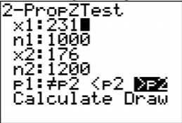
Do husbands cheat on their wives more than wives cheat on their husbands ("Statistics brain," 2013)? Suppose you take a group of 1000 randomly selected husbands and find that 231 had cheated on their wives. Suppose in a group of 1200 randomly selected wives, 176 cheated on their husbands. Do the data show that the proportion of husbands who cheat on their wives are more than the proportion of wives who cheat on their husbands. Test at the 5% level.

State the random variables and the parameters in words.
State the null and alternative hypotheses and the level of significance.
State and check the assumptions for a hypothesis test.
Find the sample statistics, test statistic, and p-value.
Conclusion
Interpretation

Solution

1. $x_{1}$ = number of husbands who cheat on his wife

$x_{2}$ = number of wives who cheat on her husband

$p_{1}$ = proportion of husbands who cheat on his wife

$p_{2}$ = proportion of wives who cheat on her husband

2. $\begin{array}{ll}{H_{o} : p_{1}=p_{2}} & {\text { or } \quad H_{o} : p_{1}-p_{2}=0} \\ {H_{A} : p_{1}>p_{2}} &\quad\quad\: {H_{A} : p_{1}-p_{2}>0} \\ {a=0.05}\end{array}$

A simple random sample of 1000 responses about cheating from husbands is taken. This was stated in the problem. A simple random sample of 1200 responses about cheating from wives is taken. This was stated in the problem.
The samples are independent. This is true since the samples involved different genders.
The properties of the binomial distribution are satisfied in both populations. This is true since there are only two responses, there are a fixed number of trials, the probability of a success is the same, and the trials are independent.
The sampling distributions of $\hat{p}_{1}$ and $\hat{p}_{2}$ can be approximated with a normal distribution.
$x_{1}=231, n_{1}-x_{1}=1000-231=769, x_{2}=176$ , and
$n_{2}-x_{2}=1200-176=1024$ are all greater than or equal to 5. So both sampling distributions of $\hat{p}_{1}$ and $\hat{p}_{2}$ can be approximated with a normal distribution.

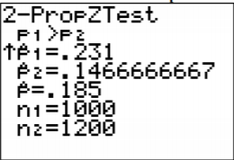
4. Sample Proportion:

$\begin{array}{ll}{n_{1}=1000} & {n_{2}=1200} \\ {\hat{p}_{1}=\dfrac{231}{1000}=0.231} & {\hat{p}_{2}=\dfrac{176}{1200} \approx 0.1467} \\ {\hat{q}_{1}=1-\dfrac{231}{1000}=\dfrac{769}{1000}=0.769} & {\hat{q}_{2}=1-\dfrac{176}{1200}=\dfrac{1024}{1200} \approx 0.8533}\end{array}$

Pooled Sample Proportion, $\overline{p}$ :

$\begin{array}{l}{\overline{p}=\dfrac{231+176}{1000+1200}=\dfrac{407}{2200}=0.185} \\ {\overline{q}=1-\dfrac{407}{2200}=\dfrac{1793}{2200}=0.815}\end{array}$

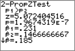
Test Statistic:

$z=\dfrac{(0.231-0.1467)-0}{\sqrt{\dfrac{0.185 * 0.815}{1000}+\dfrac{0.185 * 0.815}{1200}}}$

$=5.0704$

p-value:

On TI-83/84: normalcdf $(5.0704,1 E 99,0,1)=1.988 \times 10^{-7}$

On R: $1-\text { pnorm }(5.0704,0,1)=1.988 \times 10^{-7}$

Screenshot (158).png — Figure $\PageIndex{1}$ : Setup for 2-PropZTest on TI-83/84 Calculator

Screenshot (159).png — Figure $\PageIndex{2}$ : Results for 2-PropZTest on TI-83/84 Calculator

Screenshot (160).png — Figure $\PageIndex{3}$ : Results for 2-PropZTest on TI-83/84: Calculator

On R: prop.test $\left(c\left(x_{1}, x_{2}\right), c\left(n_{1}, n_{2}\right), \text { alternative }=\right.$ "less" or "greater". For this example, prop.test(c(231,176), c(1000, 1200), alternative="greater")

2-sample test for equality of proportions with continuity correction

data: c(231, 176) out of c(1000, 1200)

X-squared = 25.173, df = 1, p-value = 2.621e-07

alternative hypothesis: greater

95 percent confidence interval:

0.05579805 1.00000000

sample estimates:

prop 1 prop 2

0.2310000 0.1466667

Note

Again, computer software may do a continuity correction here, leading to a slightly different answer.

5. Conclusion

Reject $H_{o}$ , since the p-value is less than 5%.

6. Interpretation This is enough evidence to show that the proportion of husbands having affairs is more than the proportion of wives having affairs.

Example $\PageIndex{2}$ confidence interval for two population properties

Do more husbands cheat on their wives more than wives cheat on the husbands ("Statistics brain," 2013)? Suppose you take a group of 1000 randomly selected husbands and find that 231 had cheated on their wives. Suppose in a group of 1200 randomly selected wives, 176 cheated on their husbands. Estimate the difference in the proportion of husbands and wives who cheat on their spouses using a 95% confidence level.

State the random variables and the parameters in words.
State and check the assumptions for the confidence interval.
Find the sample statistics and the confidence interval.
Statistical Interpretation
Real World Interpretation

Solution

1. These were stated in Example $\PageIndex{1}$ , but are reproduced here for reference.

$x_{1}$ = number of husbands who cheat on his wife

$x_{2}$ = number of wives who cheat on her husband

$p_{1}$ = proportion of husbands who cheat on his wife

$p_{2}$ = proportion of wives who cheat on her husband

2. The assumptions were stated and checked in Example $\PageIndex{1}$ .

3. Sample Proportion:

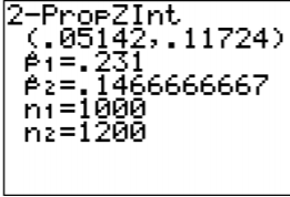
Confidence Interval:

$\begin{array}{l}{z_{c}=1.96} \\ {E=1.96 \sqrt{\dfrac{0.231 * 0.769}{1000}+\dfrac{0.1467 * 0.8533}{1200}}=0.033}\end{array}$

The confidence interval estimate of the difference $p_{1}-p_{2}$ is

$\begin{array}{l}{\left(\hat{p}_{1}-\hat{p}_{2}\right)-E<p_{1}-p_{2}<\left(\hat{p}_{1}-\hat{p}_{2}\right)+E} \\ {(0.231-0.1467)-0.033<p_{1}-p_{2}<(0.231-0.1467)+0.033} \\ {0.0513<p_{1}-p_{2}<0.1173}\end{array}$

Screenshot (161).png — Figure 9.1.4: Setup for 2-PropZInt on TI-83/84 Calculator

Screenshot (162).png — Figure $\PageIndex{5}$ : Results for 2-PropZInt on TI-83/84 Calculator

On R: prop.test $\left(c\left(x_{1}, x_{2}\right), c\left(n_{1}, n_{2}\right), \text { conf.level }=\mathrm{C}\right)$ , where C is in decimal form. For this example, prop.test(c(231,176), c(1000, 1200), conf.level=0.95)

2-sample test for equality of proportions with continuity correction

data: c(231, 176) out of c(1000, 1200)

X-squared = 25.173, df = 1, p-value = 5.241e-07

alternative hypothesis: two.sided

95 percent confidence interval:

0.05050705 0.11815962

sample estimates:

prop 1 prop 2

0.2310000 0.1466667

4. Statistical Interpretation: There is a 95% chance that $0.0505<p_{1}-p_{2}<0.1182$ contains the true difference in proportions.

5. Real World Interpretation: The proportion of husbands who cheat is anywhere from 5.05% to 11.82% higher than the proportion of wives who cheat.

Homework

Exercise $\PageIndex{1}$

In each problem show all steps of the hypothesis test or confidence interval. If some of the assumptions are not met, note that the results of the test or interval may not be correct and then continue the process of the hypothesis test or confidence interval.

Many high school students take the AP tests in different subject areas. In 2007, of the 144,796 students who took the biology exam 84,199 of them were female. In that same year, of the 211,693 students who took the calculus AB exam 102,598 of them were female ("AP exam scores," 2013). Is there enough evidence to show that the proportion of female students taking the biology exam is higher than the proportion of female students taking the calculus AB exam? Test at the 5% level.
Many high school students take the AP tests in different subject areas. In 2007, of the 144,796 students who took the biology exam 84,199 of them were female. In that same year, of the 211,693 students who took the calculus AB exam 102,598 of them were female ("AP exam scores," 2013). Estimate the difference in the proportion of female students taking the biology exam and female students taking the calculus AB exam using a 90% confidence level.
Many high school students take the AP tests in different subject areas. In 2007, of the 211,693 students who took the calculus AB exam 102,598 of them were female and 109,095 of them were male ("AP exam scores," 2013). Is there enough evidence to show that the proportion of female students taking the calculus AB exam is different from the proportion of male students taking the calculus AB exam? Test at the 5% level.
Many high school students take the AP tests in different subject areas. In 2007, of the 211,693 students who took the calculus AB exam 102,598 of them were female and 109,095 of them were male ("AP exam scores," 2013). Estimate using a 90% level the difference in proportion of female students taking the calculus AB exam versus male students taking the calculus AB exam.
Are there more children diagnosed with Autism Spectrum Disorder (ASD) in states that have larger urban areas over states that are mostly rural? In the state of Pennsylvania, a fairly urban state, there are 245 eight year olds diagnosed with ASD out of 18,440 eight year olds evaluated. In the state of Utah, a fairly rural state, there are 45 eight year olds diagnosed with ASD out of 2,123 eight year olds evaluated ("Autism and developmental," 2008). Is there enough evidence to show that the proportion of children diagnosed with ASD in Pennsylvania is more than the proportion in Utah? Test at the 1% level.
Are there more children diagnosed with Autism Spectrum Disorder (ASD) in states that have larger urban areas over states that are mostly rural? In the state of Pennsylvania, a fairly urban state, there are 245 eight year olds diagnosed with ASD out of 18,440 eight year olds evaluated. In the state of Utah, a fairly rural state, there are 45 eight year olds diagnosed with ASD out of 2,123 eight year olds evaluated ("Autism and developmental," 2008). Estimate the difference in proportion of children diagnosed with ASD between Pennsylvania and Utah. Use a 98% confidence level.
A child dying from an accidental poisoning is a terrible incident. Is it more likely that a male child will get into poison than a female child? To find this out, data was collected that showed that out of 1830 children between the ages one and four who pass away from poisoning, 1031 were males and 799 were females (Flanagan, Rooney & Griffiths, 2005). Do the data show that there are more male children dying of poisoning than female children? Test at the 1% level.
A child dying from an accidental poisoning is a terrible incident. Is it more likely that a male child will get into poison than a female child? To find this out, data was collected that showed that out of 1830 children between the ages one and four who pass away from poisoning, 1031 were males and 799 were females (Flanagan, Rooney & Griffiths, 2005). Compute a 99% confidence interval for the difference in proportions of poisoning deaths of male and female children ages one to four.

Answer

For all hypothesis tests, just the conclusion is given. For all confidence intervals, just the interval using technology (Software R) is given. See solution for the entire answer.

Reject Ho
$0.0941<p_{1}-p_{2}<0.0996$
Reject Ho
$-0.0332<p_{1}-p_{2}<-0.0282$
Fail to reject Ho
$-0.01547<p_{1}-p_{2}<-0.0001$
Reject Ho
$0.0840<p_{1}-p_{2}<0.1696$

Hypothesis Test for Two Populations Proportion (2-Prop Test)

Confidence Interval for the Difference Between Two Population Proportion (2-Prop Interval)

Homework

Support Center

How can we help?