8.2: One-Sample Interval for the Proportion
- Page ID
- 16365
\( \newcommand{\vecs}[1]{\overset { \scriptstyle \rightharpoonup} {\mathbf{#1}} } \)
\( \newcommand{\vecd}[1]{\overset{-\!-\!\rightharpoonup}{\vphantom{a}\smash {#1}}} \)
\( \newcommand{\id}{\mathrm{id}}\) \( \newcommand{\Span}{\mathrm{span}}\)
( \newcommand{\kernel}{\mathrm{null}\,}\) \( \newcommand{\range}{\mathrm{range}\,}\)
\( \newcommand{\RealPart}{\mathrm{Re}}\) \( \newcommand{\ImaginaryPart}{\mathrm{Im}}\)
\( \newcommand{\Argument}{\mathrm{Arg}}\) \( \newcommand{\norm}[1]{\| #1 \|}\)
\( \newcommand{\inner}[2]{\langle #1, #2 \rangle}\)
\( \newcommand{\Span}{\mathrm{span}}\)
\( \newcommand{\id}{\mathrm{id}}\)
\( \newcommand{\Span}{\mathrm{span}}\)
\( \newcommand{\kernel}{\mathrm{null}\,}\)
\( \newcommand{\range}{\mathrm{range}\,}\)
\( \newcommand{\RealPart}{\mathrm{Re}}\)
\( \newcommand{\ImaginaryPart}{\mathrm{Im}}\)
\( \newcommand{\Argument}{\mathrm{Arg}}\)
\( \newcommand{\norm}[1]{\| #1 \|}\)
\( \newcommand{\inner}[2]{\langle #1, #2 \rangle}\)
\( \newcommand{\Span}{\mathrm{span}}\) \( \newcommand{\AA}{\unicode[.8,0]{x212B}}\)
\( \newcommand{\vectorA}[1]{\vec{#1}} % arrow\)
\( \newcommand{\vectorAt}[1]{\vec{\text{#1}}} % arrow\)
\( \newcommand{\vectorB}[1]{\overset { \scriptstyle \rightharpoonup} {\mathbf{#1}} } \)
\( \newcommand{\vectorC}[1]{\textbf{#1}} \)
\( \newcommand{\vectorD}[1]{\overrightarrow{#1}} \)
\( \newcommand{\vectorDt}[1]{\overrightarrow{\text{#1}}} \)
\( \newcommand{\vectE}[1]{\overset{-\!-\!\rightharpoonup}{\vphantom{a}\smash{\mathbf {#1}}}} \)
\( \newcommand{\vecs}[1]{\overset { \scriptstyle \rightharpoonup} {\mathbf{#1}} } \)
\( \newcommand{\vecd}[1]{\overset{-\!-\!\rightharpoonup}{\vphantom{a}\smash {#1}}} \)
\(\newcommand{\avec}{\mathbf a}\) \(\newcommand{\bvec}{\mathbf b}\) \(\newcommand{\cvec}{\mathbf c}\) \(\newcommand{\dvec}{\mathbf d}\) \(\newcommand{\dtil}{\widetilde{\mathbf d}}\) \(\newcommand{\evec}{\mathbf e}\) \(\newcommand{\fvec}{\mathbf f}\) \(\newcommand{\nvec}{\mathbf n}\) \(\newcommand{\pvec}{\mathbf p}\) \(\newcommand{\qvec}{\mathbf q}\) \(\newcommand{\svec}{\mathbf s}\) \(\newcommand{\tvec}{\mathbf t}\) \(\newcommand{\uvec}{\mathbf u}\) \(\newcommand{\vvec}{\mathbf v}\) \(\newcommand{\wvec}{\mathbf w}\) \(\newcommand{\xvec}{\mathbf x}\) \(\newcommand{\yvec}{\mathbf y}\) \(\newcommand{\zvec}{\mathbf z}\) \(\newcommand{\rvec}{\mathbf r}\) \(\newcommand{\mvec}{\mathbf m}\) \(\newcommand{\zerovec}{\mathbf 0}\) \(\newcommand{\onevec}{\mathbf 1}\) \(\newcommand{\real}{\mathbb R}\) \(\newcommand{\twovec}[2]{\left[\begin{array}{r}#1 \\ #2 \end{array}\right]}\) \(\newcommand{\ctwovec}[2]{\left[\begin{array}{c}#1 \\ #2 \end{array}\right]}\) \(\newcommand{\threevec}[3]{\left[\begin{array}{r}#1 \\ #2 \\ #3 \end{array}\right]}\) \(\newcommand{\cthreevec}[3]{\left[\begin{array}{c}#1 \\ #2 \\ #3 \end{array}\right]}\) \(\newcommand{\fourvec}[4]{\left[\begin{array}{r}#1 \\ #2 \\ #3 \\ #4 \end{array}\right]}\) \(\newcommand{\cfourvec}[4]{\left[\begin{array}{c}#1 \\ #2 \\ #3 \\ #4 \end{array}\right]}\) \(\newcommand{\fivevec}[5]{\left[\begin{array}{r}#1 \\ #2 \\ #3 \\ #4 \\ #5 \\ \end{array}\right]}\) \(\newcommand{\cfivevec}[5]{\left[\begin{array}{c}#1 \\ #2 \\ #3 \\ #4 \\ #5 \\ \end{array}\right]}\) \(\newcommand{\mattwo}[4]{\left[\begin{array}{rr}#1 \amp #2 \\ #3 \amp #4 \\ \end{array}\right]}\) \(\newcommand{\laspan}[1]{\text{Span}\{#1\}}\) \(\newcommand{\bcal}{\cal B}\) \(\newcommand{\ccal}{\cal C}\) \(\newcommand{\scal}{\cal S}\) \(\newcommand{\wcal}{\cal W}\) \(\newcommand{\ecal}{\cal E}\) \(\newcommand{\coords}[2]{\left\{#1\right\}_{#2}}\) \(\newcommand{\gray}[1]{\color{gray}{#1}}\) \(\newcommand{\lgray}[1]{\color{lightgray}{#1}}\) \(\newcommand{\rank}{\operatorname{rank}}\) \(\newcommand{\row}{\text{Row}}\) \(\newcommand{\col}{\text{Col}}\) \(\renewcommand{\row}{\text{Row}}\) \(\newcommand{\nul}{\text{Nul}}\) \(\newcommand{\var}{\text{Var}}\) \(\newcommand{\corr}{\text{corr}}\) \(\newcommand{\len}[1]{\left|#1\right|}\) \(\newcommand{\bbar}{\overline{\bvec}}\) \(\newcommand{\bhat}{\widehat{\bvec}}\) \(\newcommand{\bperp}{\bvec^\perp}\) \(\newcommand{\xhat}{\widehat{\xvec}}\) \(\newcommand{\vhat}{\widehat{\vvec}}\) \(\newcommand{\uhat}{\widehat{\uvec}}\) \(\newcommand{\what}{\widehat{\wvec}}\) \(\newcommand{\Sighat}{\widehat{\Sigma}}\) \(\newcommand{\lt}{<}\) \(\newcommand{\gt}{>}\) \(\newcommand{\amp}{&}\) \(\definecolor{fillinmathshade}{gray}{0.9}\)Suppose you want to estimate the population proportion, p. As an example you may be curious what proportion of students at your school smoke. Or you could wonder what is the proportion of accidents caused by teenage drivers who do not have a drivers’ education class.
Confidence Interval for One Population Proportion (1-Prop Interval)
- State the random variable and the parameter in words.
x = number of successes
p = proportion of successes - State and check the assumptions for confidence interval
- A simple random sample of size n is taken.
- The condition for the binomial distribution are satisfied
- To determine the sampling distribution of \(\hat{p}\), you need to show that \(n \hat{p} \geq 5\) and \(n \hat{q} \geq 5\), where \(\hat{q}=1-\hat{p}\). If this requirement is true, then the sampling distribution of \(\hat{p}\) is well approximated by a normal curve. (In reality this is not really true, since the correct assumption deals with p. However, in a confidence interval you do not know p, so you must use \(\hat{p}\). This means you just need to show that \(x \geq 5\) and \(n-x \geq 5\).)
- Find the sample statistic and the confidence interval
Sample Proportion:
\(\hat{p}=\dfrac{x}{n}=\dfrac{\# \text { of successes }}{\# \text { of trials }}\)
Confidence Interval:
\(\hat{p}-E<p<\hat{p}+E\)
Where
p = population proportion
\(\hat{p}\) = sample proportion
n = number of sample values
E = margin of error
\(z_{c}=\) = critical value
\(\hat{q}=1-\hat{p}\)
\(E=z_{c} \sqrt{\dfrac{\hat{p} \hat{q}}{n}}\) - Statistical Interpretation: In general this looks like, “there is a C% chance that \(\hat{p}-E<p<\hat{p}+E\) contains the true proportion.”
- Real World Interpretation: This is where you state what interval contains the true proportion.
The critical value is a value from the normal distribution. Since a confidence interval is found by adding and subtracting a margin of error amount from the sample proportion, and the interval has a probability of containing the true proportion, then you can think of this as the statement \(P(\hat{p}-E<p<\hat{p}+E)=C\). You can use the invNorm command on the TI-83/84 calculator to find the critical value. The critical values will always be the same value, so it is easier to just look at table A.1 in the appendix.
Example \(\PageIndex{1}\) confidence interval for the population proportion using the formula
A concern was raised in Australia that the percentage of deaths of Aboriginal prisoners was higher than the percent of deaths of non-Aboriginal prisoners, which is 0.27%. A sample of six years (1990-1995) of data was collected, and it was found that out of 14,495 Aboriginal prisoners, 51 died ("Indigenous deaths in," 1996). Find a 95% confidence interval for the proportion of Aboriginal prisoners who died.
- State the random variable and the parameter in words.
- State and check the assumptions for a confidence interval.
- Find the sample statistic and the confidence interval.
- Statistical Interpretation
- Real World Interpretation
Solution
1. x = number of Aboriginal prisoners who die
p = proportion of Aboriginal prisoners who die
2.
- A simple random sample of 14,495 Aboriginal prisoners was taken. However, the sample was not a random sample, since it was data from six years. It is the numbers for all prisoners in these six years, but the six years were not picked at random. Unless there was something special about the six years that were chosen, the sample is probably a representative sample. This assumption is probably met.
- There are 14,495 prisoners in this case. The prisoners are all Aboriginals, so you are not mixing Aboriginal with non-Aboriginal prisoners. There are only two outcomes, either the prisoner dies or doesn’t. The chance that one prisoner dies over another may not be constant, but if you consider all prisoners the same, then it may be close to the same probability. Thus the assumptions for the binomial distribution are satisfied
- In this case, x = 51 and n - x = 14495 - 51 = 14444 and both are greater than or equal to 5. The sampling distribution for \(\hat{p}\) is a normal distribution.
3. Sample Proportion:
\(\hat{p}=\dfrac{x}{n}=\dfrac{51}{14495} \approx 0.003518\)
Confidence Interval:
\(z_{c}=1.96\), since 95% confidence level
\(E=z_{c} \sqrt{\dfrac{\hat{p} \hat{q}}{n}}=1.96 \sqrt{\dfrac{0.003518(1-0.003518)}{14495}} \approx 0.000964\)
\(\hat{p}-E<p<\hat{p}+E\)
\(0.003518-0.000964<p<0.003518+0.000964\)
\(0.002554<p<0.004482\)
4. There is a 95% chance that \(0.002554<p<0.004482\) contains the proportion of Aboriginal prisoners who died.
5. The proportion of Aboriginal prisoners who died is between 0.0026 and 0.0045.
You can also do the calculations for the confidence interval with technology. The following example shows the process on the TI-83/84.
Example \(\PageIndex{2}\) confidence interval for the population proportion using technology
A researcher studying the effects of income levels on breastfeeding of infants hypothesizes that countries where the income level is lower have a higher rate of infant breastfeeding than higher income countries. It is known that in Germany, considered a high-income country by the World Bank, 22% of all babies are breastfeed. In Tajikistan, considered a low-income country by the World Bank, researchers found that in a random sample of 500 new mothers that 125 were breastfeeding their infants. Find a 90% confidence interval of the proportion of mothers in low-income countries who breastfeed their infants?
- State you random variable and the parameter in words.
- State and check the assumptions for a confidence interval.
- Find the sample statistic and the confidence interval.
- Statistical Interpretation
- Real World Interpretation
Solution
1. x = number of woman who breastfeed in a low-income country
p = proportion of woman who breastfeed in a low-income country
2.
- A simple random sample of 500 breastfeeding habits of woman in a low-income country was taken as was stated in the problem.
- There were 500 women in the study. The women are considered identical, though they probably have some differences. There are only two outcomes, either the woman breastfeeds or she doesn’t. The probability of a woman breastfeeding is probably not the same for each woman, but it is probably not very different for each woman. The assumptions for the binomial distribution are satisfied
- x = 125 and n - x = 500 - 125 = 375 and both are greater than or equal to 5, so the sampling distribution of \(\hat{p}\) is well approximated by a normal curve.
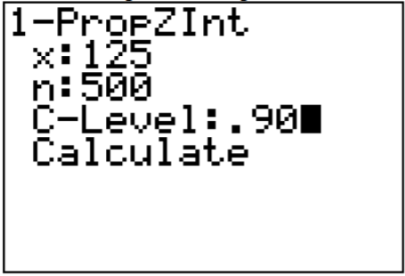
3. On the TI-83/84: Go into the STAT menu. Move over to TESTS and choose 1-PropZInt.
.png?revision=1)
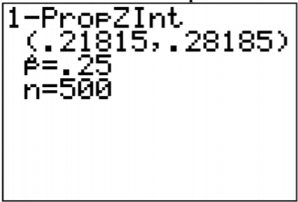
Once you press Calculate, you will see the results as in Figure \(\PageIndex{2}\).
.png?revision=1)
On R: the command is prop.test(x, n, conf.level = C), where C is given in decimal form. So for this example, the command is
prop.test(125, 500, conf.level = 0.90)
1-sample proportions test with continuity correction
data: 125 out of 500, null probability 0.5
X-squared = 124, df = 1, p-value < 2.2e-16
alternative hypothesis: true p is not equal to 0.5
90 percent confidence interval:
0.2185980 0.2841772
sample estimates:
p
0.25
Some software does a continuity correction, so the answer can be slightly off from the formula and the TI-83/84 calculator.
0.219 < p < 0.284
4. There is a 90% chance that 0.219 < p < 0.284 contains the proportion of women in low-income countries who breastfeed their infants.
5. The proportion of women in low-income countries who breastfeed their infants is between 0.219 and 0.284.
Homework
Exercise \(\PageIndex{1}\)
In each problem show all steps of the confidence interval. If some of the assumptions are not met, note that the results of the interval may not be correct and then continue the process of the confidence interval.
- Eyeglassomatic manufactures eyeglasses for different retailers. They test to see how many defective lenses they make. Looking at the type of defects, they found in a three-month time period that out of 34,641 defective lenses, 5865 were due to scratches. Find a 99% confidence interval for the proportion of defects that are from scratches.
- In November of 1997, Australians were asked if they thought unemployment would increase. At that time 284 out of 631 said that they thought unemployment would increase ("Morgan gallup poll," 2013). Estimate the proportion of Australians in November 1997 who believed unemployment would increase using a 95% confidence interval?
- According to the February 2008 Federal Trade Commission report on consumer fraud and identity theft, Arkansas had 1,601 complaints of identity theft out of 3,482 consumer complaints ("Consumer fraud and," 2008). Calculate a 90% confidence interval for the proportion of identity theft in Arkansas.
- According to the February 2008 Federal Trade Commission report on consumer fraud and identity theft, Alaska had 321 complaints of identity theft out of 1,432 consumer complaints ("Consumer fraud and," 2008). Calculate a 90% confidence interval for the proportion of identity theft in Alaska.
- In 2013, the Gallup poll asked 1,039 American adults if they believe there was a conspiracy in the assassination of President Kennedy, and found that 634 believe there was a conspiracy ("Gallup news service," 2013). Estimate the proportion of American’s who believe in this conspiracy using a 98% confidence interval.
- In 2008, there were 507 children in Arizona out of 32,601 who were diagnosed with Autism Spectrum Disorder (ASD) ("Autism and developmental," 2008). Find the proportion of ASD in Arizona with a confidence level of 99%.
- Answer
-
For all confidence intervals, just the interval using technology is given. See solution for the entire answer.
1. 0.1641 < p < 0.1745
3. 0.4458 < p < 0.4739
5. 0.5740 < p < 0.6452


