3.1: Measures of Center
- Page ID
- 16341
\( \newcommand{\vecs}[1]{\overset { \scriptstyle \rightharpoonup} {\mathbf{#1}} } \)
\( \newcommand{\vecd}[1]{\overset{-\!-\!\rightharpoonup}{\vphantom{a}\smash {#1}}} \)
\( \newcommand{\dsum}{\displaystyle\sum\limits} \)
\( \newcommand{\dint}{\displaystyle\int\limits} \)
\( \newcommand{\dlim}{\displaystyle\lim\limits} \)
\( \newcommand{\id}{\mathrm{id}}\) \( \newcommand{\Span}{\mathrm{span}}\)
( \newcommand{\kernel}{\mathrm{null}\,}\) \( \newcommand{\range}{\mathrm{range}\,}\)
\( \newcommand{\RealPart}{\mathrm{Re}}\) \( \newcommand{\ImaginaryPart}{\mathrm{Im}}\)
\( \newcommand{\Argument}{\mathrm{Arg}}\) \( \newcommand{\norm}[1]{\| #1 \|}\)
\( \newcommand{\inner}[2]{\langle #1, #2 \rangle}\)
\( \newcommand{\Span}{\mathrm{span}}\)
\( \newcommand{\id}{\mathrm{id}}\)
\( \newcommand{\Span}{\mathrm{span}}\)
\( \newcommand{\kernel}{\mathrm{null}\,}\)
\( \newcommand{\range}{\mathrm{range}\,}\)
\( \newcommand{\RealPart}{\mathrm{Re}}\)
\( \newcommand{\ImaginaryPart}{\mathrm{Im}}\)
\( \newcommand{\Argument}{\mathrm{Arg}}\)
\( \newcommand{\norm}[1]{\| #1 \|}\)
\( \newcommand{\inner}[2]{\langle #1, #2 \rangle}\)
\( \newcommand{\Span}{\mathrm{span}}\) \( \newcommand{\AA}{\unicode[.8,0]{x212B}}\)
\( \newcommand{\vectorA}[1]{\vec{#1}} % arrow\)
\( \newcommand{\vectorAt}[1]{\vec{\text{#1}}} % arrow\)
\( \newcommand{\vectorB}[1]{\overset { \scriptstyle \rightharpoonup} {\mathbf{#1}} } \)
\( \newcommand{\vectorC}[1]{\textbf{#1}} \)
\( \newcommand{\vectorD}[1]{\overrightarrow{#1}} \)
\( \newcommand{\vectorDt}[1]{\overrightarrow{\text{#1}}} \)
\( \newcommand{\vectE}[1]{\overset{-\!-\!\rightharpoonup}{\vphantom{a}\smash{\mathbf {#1}}}} \)
\( \newcommand{\vecs}[1]{\overset { \scriptstyle \rightharpoonup} {\mathbf{#1}} } \)
\( \newcommand{\vecd}[1]{\overset{-\!-\!\rightharpoonup}{\vphantom{a}\smash {#1}}} \)
\(\newcommand{\avec}{\mathbf a}\) \(\newcommand{\bvec}{\mathbf b}\) \(\newcommand{\cvec}{\mathbf c}\) \(\newcommand{\dvec}{\mathbf d}\) \(\newcommand{\dtil}{\widetilde{\mathbf d}}\) \(\newcommand{\evec}{\mathbf e}\) \(\newcommand{\fvec}{\mathbf f}\) \(\newcommand{\nvec}{\mathbf n}\) \(\newcommand{\pvec}{\mathbf p}\) \(\newcommand{\qvec}{\mathbf q}\) \(\newcommand{\svec}{\mathbf s}\) \(\newcommand{\tvec}{\mathbf t}\) \(\newcommand{\uvec}{\mathbf u}\) \(\newcommand{\vvec}{\mathbf v}\) \(\newcommand{\wvec}{\mathbf w}\) \(\newcommand{\xvec}{\mathbf x}\) \(\newcommand{\yvec}{\mathbf y}\) \(\newcommand{\zvec}{\mathbf z}\) \(\newcommand{\rvec}{\mathbf r}\) \(\newcommand{\mvec}{\mathbf m}\) \(\newcommand{\zerovec}{\mathbf 0}\) \(\newcommand{\onevec}{\mathbf 1}\) \(\newcommand{\real}{\mathbb R}\) \(\newcommand{\twovec}[2]{\left[\begin{array}{r}#1 \\ #2 \end{array}\right]}\) \(\newcommand{\ctwovec}[2]{\left[\begin{array}{c}#1 \\ #2 \end{array}\right]}\) \(\newcommand{\threevec}[3]{\left[\begin{array}{r}#1 \\ #2 \\ #3 \end{array}\right]}\) \(\newcommand{\cthreevec}[3]{\left[\begin{array}{c}#1 \\ #2 \\ #3 \end{array}\right]}\) \(\newcommand{\fourvec}[4]{\left[\begin{array}{r}#1 \\ #2 \\ #3 \\ #4 \end{array}\right]}\) \(\newcommand{\cfourvec}[4]{\left[\begin{array}{c}#1 \\ #2 \\ #3 \\ #4 \end{array}\right]}\) \(\newcommand{\fivevec}[5]{\left[\begin{array}{r}#1 \\ #2 \\ #3 \\ #4 \\ #5 \\ \end{array}\right]}\) \(\newcommand{\cfivevec}[5]{\left[\begin{array}{c}#1 \\ #2 \\ #3 \\ #4 \\ #5 \\ \end{array}\right]}\) \(\newcommand{\mattwo}[4]{\left[\begin{array}{rr}#1 \amp #2 \\ #3 \amp #4 \\ \end{array}\right]}\) \(\newcommand{\laspan}[1]{\text{Span}\{#1\}}\) \(\newcommand{\bcal}{\cal B}\) \(\newcommand{\ccal}{\cal C}\) \(\newcommand{\scal}{\cal S}\) \(\newcommand{\wcal}{\cal W}\) \(\newcommand{\ecal}{\cal E}\) \(\newcommand{\coords}[2]{\left\{#1\right\}_{#2}}\) \(\newcommand{\gray}[1]{\color{gray}{#1}}\) \(\newcommand{\lgray}[1]{\color{lightgray}{#1}}\) \(\newcommand{\rank}{\operatorname{rank}}\) \(\newcommand{\row}{\text{Row}}\) \(\newcommand{\col}{\text{Col}}\) \(\renewcommand{\row}{\text{Row}}\) \(\newcommand{\nul}{\text{Nul}}\) \(\newcommand{\var}{\text{Var}}\) \(\newcommand{\corr}{\text{corr}}\) \(\newcommand{\len}[1]{\left|#1\right|}\) \(\newcommand{\bbar}{\overline{\bvec}}\) \(\newcommand{\bhat}{\widehat{\bvec}}\) \(\newcommand{\bperp}{\bvec^\perp}\) \(\newcommand{\xhat}{\widehat{\xvec}}\) \(\newcommand{\vhat}{\widehat{\vvec}}\) \(\newcommand{\uhat}{\widehat{\uvec}}\) \(\newcommand{\what}{\widehat{\wvec}}\) \(\newcommand{\Sighat}{\widehat{\Sigma}}\) \(\newcommand{\lt}{<}\) \(\newcommand{\gt}{>}\) \(\newcommand{\amp}{&}\) \(\definecolor{fillinmathshade}{gray}{0.9}\)This section focuses on measures of central tendency. Many times you are asking what to expect on average. Such as when you pick a major, you would probably ask how much you expect to earn in that field. If you are thinking of relocating to a new town, you might ask how much you can expect to pay for housing. If you are planting vegetables in the spring, you might want to know how long it will be until you can harvest. These questions, and many more, can be answered by knowing the center of the data set. There are three measures of the “center” of the data. They are the mode, median, and mean. Any of the values can be referred to as the “average.”
- The mode is the data value that occurs the most frequently in the data. To find it, you count how often each data value occurs, and then determine which data value occurs most often.
- The median is the data value in the middle of a sorted list of data. To find it, you put the data in order, and then determine which data value is in the middle of the data set.
- The mean is the arithmetic average of the numbers. This is the center that most people call the average, though all three – mean, median, and mode – really are averages.
There are no symbols for the mode and the median, but the mean is used a great deal, and statisticians gave it a symbol. There are actually two symbols, one for the population parameter and one for the sample statistic. In most cases you cannot find the population parameter, so you use the sample statistic to estimate the population parameter.
Definition \(\PageIndex{1}\): Population Mean
The population mean is given by
\(\mu=\dfrac{\sum x}{N}\), pronounced mu
where
- \(N\) is the size of the population.
- \(x\) represents a data value.
- \(\sum x\) means to add up all of the data values.
Definition \(\PageIndex{2}\): Sample Mean
Sample Mean:
\(\overline{x}=\dfrac{\sum x}{n}\), pronounced x bar, where
- \(n\) is the size of the sample.
- \(x\) represents a data value.
- \(\sum x\) means to add up all of the data values.
The value for \(\overline{x}\) is used to estimate \(\mu\) since \(\mu\) can't be calculated in most situations.
Example \(\PageIndex{1}\) finding the mean, median, and mode
Suppose a vet wants to find the average weight of cats. The weights (in pounds) of five cats are in Example \(\PageIndex{1}\).
| 6.8 | 8.2 | 7.5 | 9.4 | 8.2 |
Find the mean, median, and mode of the weight of a cat.
Solution
Before starting any mathematics problem, it is always a good idea to define the unknown in the problem. In this case, you want to define the variable. The symbol for the variable is \(x\).
The variable is \(x =\) weight of a cat
Mean:
\(\overline{x}=\dfrac{6.8+8.2+7.5+9.4+8.2}{5}=\dfrac{40.1}{5}=8.02\) pounds
Median:
You need to sort the list for both the median and mode. The sorted list is in Example \(\PageIndex{2}\).
| 6.8 | 7.5 | 8.2 | 8.2 | 9.4 |
There are 5 data points so the middle of the list would be the 3rd number. (Just put a finger at each end of the list and move them toward the center one number at a time. Where your fingers meet is the median.)
| 6.8 | 7.5 | 8.2 | 8.2 | 9.4 |
The median is therefore 8.2 pounds.
Mode:
This is easiest to do from the sorted list that is in Example \(\PageIndex{2}\). Which value appears the most number of times? The number 8.2 appears twice, while all other numbers appear once.
Mode = 8.2 pounds.
A data set can have more than one mode. If there is a tie between two values for the most number of times then both values are the mode and the data is called bimodal (two modes). If every data point occurs the same number of times, there is no mode. If there are more than two numbers that appear the most times, then usually there is no mode.
In Example \(\PageIndex{1}\), there were an odd number of data points. In that case, the median was just the middle number. What happens if there is an even number of data points? What would you do?
Example \(\PageIndex{2}\) finding the median with an even number of data points
Suppose a vet wants to find the median weight of cats. The weights (in pounds) of six cats are in Example \(\PageIndex{4}\). Find the median.
| 6.8 | 8.2 | 7.5 | 9.4 | 8.2 | 6.3 |
Solution
Variable: \(x =\) weight of a cat
First sort the list if it is not already sorted.
There are 6 numbers in the list so the number in the middle is between the 3rd and 4th number. Use your fingers starting at each end of the list in Example \(\PageIndex{5}\) and move toward the center until they meet. There are two numbers there.
| 6.3 | 6.8 | 7.5 | 8.2 | 8.2 | 9.4 |
To find the median, just average the two numbers.
median \(=\dfrac{7.5+8.2}{2}=7.85\) pounds
The median is 7.85 pounds.
Example \(\PageIndex{3}\) finding mean and median using technology
Suppose a vet wants to find the median weight of cats. The weights (in pounds) of six cats are in Example \(\PageIndex{4}\). Find the median
Solution
Variable: \(x=\) weight of a cat
You can do the calculations for the mean and median using the technology.
The procedure for calculating the sample mean ( \(\overline{x}\) ) and the sample median (Med) on the TI-83/84 is in Figures 3.1.1 through 3.1.4. First you need to go into the STAT menu, and then Edit. This will allow you to type in your data (see Figure \(\PageIndex{1}\)).
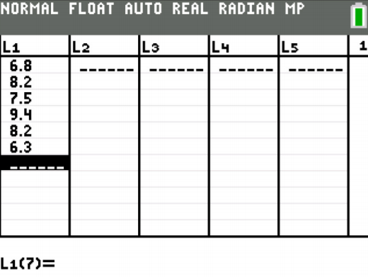.png?revision=1)
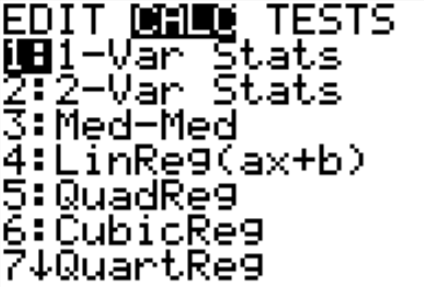
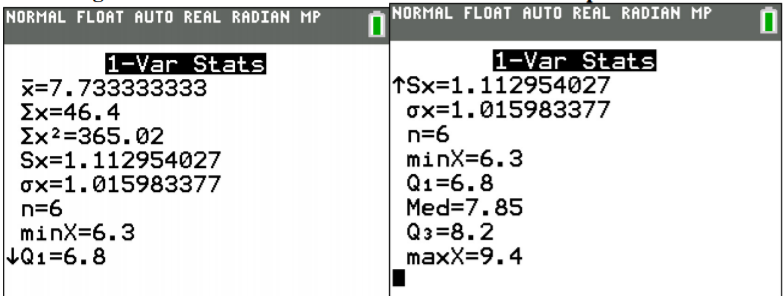
Once you have the data into the calculator, you then go back to the STAT menu, move over to CALC, and then choose 1-Var Stats (see Figure \(\PageIndex{2}\)). The calculator will now put 1-Var Stats on the main screen. Now type in L1 (2nd button and 1) and then press ENTER. (Note if you have the newer operating system on the TI-84, then the procedure is slightly different.) If you press the down arrow, you will see the rest of the output from the calculator. The results from the calculator are in Figure \(\PageIndex{3}\).
.png?revision=1)
.png?revision=1)
.png?revision=1)
Example \(\PageIndex{4}\) affect of extreme values on mean and median
Suppose you have the same set of cats from Example \(\PageIndex{1}\) but one additional cat was added to the data set. Example \(\PageIndex{6}\) contains the six cats’ weights, in pounds.
| 6.8 | 7.5 | 8.2 | 8.2 | 9.4 | 22.1 |
Find the mean and the median.
Solution
Variable: \(x=\) weight of a cat
mean \(=\overline{x}=\dfrac{6.8+7.5+8.2+8.2+9.4+22.1}{6}=10.37\) pounds
The data is already in order, thus the median is between 8.2 and 8.2.
median \(=\dfrac{8.2+8.2}{2}=8.2\) pounds
The mean is much higher than the median. Why is this? Notice that when the value of 22.1 was added, the mean went from 8.02 to 10.37, but the median did not change at all. This is because the mean is affected by extreme values, while the median is not. The very heavy cat brought the mean weight up. In this case, the median is a much better measure of the center.
An outlier is a data value that is very different from the rest of the data. It can be really high or really low. Extreme values may be an outlier if the extreme value is far enough from the center. In Example \(\PageIndex{4}\), the data value 22.1 pounds is an extreme value and it may be an outlier.
If there are extreme values in the data, the median is a better measure of the center than the mean. If there are no extreme values, the mean and the median will be similar so most people use the mean.
The mean is not a resistant measure because it is affected by extreme values. The median and the mode are resistant measures because they are not affected by extreme values.
As a consumer you need to be aware that people choose the measure of center that best supports their claim. When you read an article in the newspaper and it talks about the “average” it usually means the mean but sometimes it refers to the median. Some articles will use the word “median” instead of “average” to be more specific. If you need to make an important decision and the information says “average”, it would be wise to ask if the “average” is the mean or the median before you decide.
As an example, suppose that a company wants to use the mean salary as the average salary for the company. This is because the high salaries of the administration will pull the mean higher. The company can say that the employees are paid well because the average is high. However, the employees want to use the median since it discounts the extreme values of the administration and will give a lower value of the average. This will make the salaries seem lower and that a raise is in order.
Why use the mean instead of the median? The reason is because when multiple samples are taken from the same population, the sample means tend to be more consistent than other measures of the center. The sample mean is the more reliable measure of center.
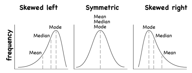
To understand how the different measures of center related to skewed or symmetric distributions, see Figure \(\PageIndex{5}\). As you can see sometimes the mean is smaller than the median and mode, sometimes the mean is larger than the median and mode, and sometimes they are the same values.
.png?revision=1)
One last type of average is a weighted average. Weighted averages are used quite often in real life. Some teachers use them in calculating your grade in the course, or your grade on a project. Some employers use them in employee evaluations. The idea is that some activities are more important than others. As an example, a fulltime teacher at a community college may be evaluated on their service to the college, their service to the community, whether their paperwork is turned in on time, and their teaching. However, teaching is much more important than whether their paperwork is turned in on time. When the evaluation is completed, more weight needs to be given to the teaching and less to the paperwork. This is a weighted average.
Definition \(\PageIndex{3}\)
Weighted Average
\(\dfrac{\sum x w}{\sum w}\) where \(w\) is the weight of the data value, \(x\).
Example \(\PageIndex{5}\) weighted average
In your biology class, your final grade is based on several things: a lab score, scores on two major tests, and your score on the final exam. There are 100 points available for each score. The lab score is worth 15% of the course, the two exams are worth 25% of the course each, and the final exam is worth 35% of the course. Suppose you earned scores of 95 on the labs, 83 and 76 on the two exams, and 84 on the final exam. Compute your weighted average for the course.
Solution
Variable: \(x=\) score
The weighted average is \(\dfrac{\sum x w}{\sum w}=\dfrac{\text { sum of the scores times their weights }}{\text { sum of all the weights }}\)
weighted average \(=\dfrac{95(0.15)+83(0.25)+76(0.25)+84(0.35)}{0.15+0.25+0.25+0.35}=\dfrac{83.4}{1.00}=83.4 \%\)
A weighted average can be found using technology.
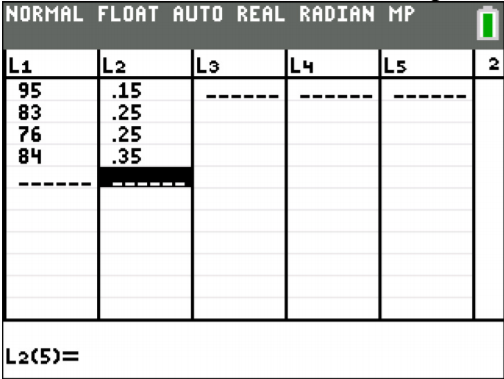
The procedure for calculating the weighted average on the TI-83/84 is in Figures 3.1.6 through 3.1.9. First you need to go into the STAT menu, and then Edit. This will allow you to type in the scores into L1 and the weights into L2 (see Figure \(\PageIndex{6}\)).
.png?revision=1)
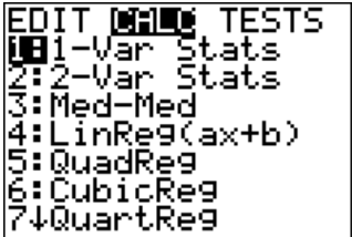
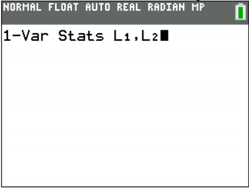
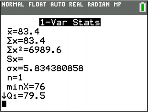
Once you have the data into the calculator, you then go back to the STAT menu, move over to CALC, and then choose 1-Var Stats (see Figure \(\PageIndex{7}\)). The calculator will now put 1-Var Stats on the main screen. Now type in L1 (2nd button and 1), then a comma (button above the 7 button), and then L2 (2nd button and 2) and then press ENTER. (Note if you have the newer operating system on the TI-84, then the procedure is slightly different.) The results from the calculator are in Figure \(\PageIndex{9}\). The \(\overline{x}\) is the weighted average.
.png?revision=1)
.png?revision=1)
.png?revision=1)
Example \(\PageIndex{6}\) weighted average
The faculty evaluation process at John Jingle University rates a faculty member on the following activities: teaching, publishing, committee service, community service, and submitting paperwork in a timely manner. The process involves reviewing student evaluations, peer evaluations, and supervisor evaluation for each teacher and awarding him/her a score on a scale from 1 to 10 (with 10 being the best). The weights for each activity are 20 for teaching, 18 for publishing, 6 for committee service, 4 for community service, and 2 for paperwork.
- One faculty member had the following ratings: 8 for teaching, 9 for publishing, 2 for committee work, 1 for community service, and 8 for paperwork. Compute the weighted average of the evaluation.
- Another faculty member had ratings of 6 for teaching, 8 for publishing, 9 for committee work, 10 for community service, and 10 for paperwork. Compute the weighted average of the evaluation.
- Which faculty member had the higher average evaluation?
Solution
a. Variable: \(x=\) rating
The weighted average is \(\dfrac{\sum x w}{\sum w}=\dfrac{\text { sum of the scores times their weights }}{\text { sum of all the weights }}\)
evaluation \(=\dfrac{8(20)+9(18)+2(6)+1(4)+8(2)}{20+18+6+4+2}=\dfrac{354}{50}=7.08\)
b. evaluation \(=\dfrac{6(20)+8(18)+9(6)+10(4)+10(2)}{20+18+6+4+2}=\dfrac{378}{50}=7.56\)
c. The second faculty member has a higher average evaluation.
You can find a weighted average using technology.
Homework
Exercise \(\PageIndex{1}\)
- Cholesterol levels were collected from patients two days after they had a heart attack (Ryan, Joiner & Ryan, Jr, 1985) and are in Example \(\PageIndex{7}\). Find the mean, median, and mode.
270 236 210 142 280 272 160 220 226 242 186 266 206 318 294 282 234 224 276 282 360 310 280 278 288 288 244 236 Table \(\PageIndex{7}\): Cholesterol Levels - The lengths (in kilometers) of rivers on the South Island of New Zealand that flow to the Pacific Ocean are listed in Example \(\PageIndex{8}\) (Lee, 1994). Find the mean, median, and mode.
River Length (km) River Length (km) Clarence 209 Clutha 322 Conway 48 Taieri 288 Waiau 169 Shag 72 Hurunui 138 Kakanui 64 Waipara 64 Rangitata 121 Ashley 97 Ophi 80 Waimakariri 161 Pareora 56 Selwyn 95 Waihao 64 Rakaia 145 Waitaki 209 Ashburton 90 Table \(\PageIndex{8}\): Lengths of Rivers (km) Flowing to Pacific Ocean - The lengths (in kilometers) of rivers on the South Island of New Zealand that flow to the Tasman Sea are listed in Example \(\PageIndex{9}\) (Lee, 1994). Find the mean, median, and mode.
River Length (km) River Length (km) Hollyford 76 Waimea 48 Cascade 64 Motueka 108 Arawhata 68 Takaka 72 Haast 64 Aorere 72 Karangarua 37 Heaphy 35 Cook 32 Karamea 80 Waiho 32 Mokihinui 56 Whataroa 51 Buller 177 Wanganui 56 Grey 121 Waitaha 40 Taramakau 80 Hokitika 64 Arahura 56 Table \(\PageIndex{9}\): Lengths of Rivers (km) Flowing to Tasman Sea - Eyeglassmatic manufactures eyeglasses for their retailers. They research to see how many defective lenses they made during the time period of January 1 to March 31. Example \(\PageIndex{10}\) contains the defect and the number of defects. Find the mean, median, and mode.
Defect Type Number of Defects Scratch 5865 Right shaped - small 4613 Flaked 1992 Wrong axis 1838 Chamfer wrong 1596 Crazing, cracks 1546 Wrong shape 1485 Wrong PD 1398 Spots and bubbles 1371 Wrong height 1130 Right shape - big 1105 Lost in lab 976 Spots/bubble - intern 976 Table \(\PageIndex{10}\): Number of Defective Lenses - Print-O-Matic printing company’s employees have salaries that are contained in Example \(\PageIndex{11}\).
Employee Salary ($) CEO 272,500 Driver 58,456 CD74 100,702 CD65 57,380 Embellisher 73,877 Folder 65,270 GTO 74,235 Handwork 52,718 Horizon 76,029 ITEK 64,553 Mgmt 108,448 Platens 69,573 Polar 75,526 Pre Press Manager 108,448 Pre Press Manager/ IT 98,837 Pre Press/ Graphic Artist 75,311 Designer 90,090 Sales 109,739 Administration 66,346 Table \(\PageIndex{11}\): Salaries of Print-O-Matic Printing Company Employees
a. Find the mean and median.
b. Find the mean and median with the CEO's salary removed.
c. What happened to the mean and median when the CEO’s salary was removed? Why?
d. If you were the CEO, who is answering concerns from the union that employees are underpaid, which average of the complete data set would you prefer? Why?
e. If you were a platen worker, who believes that the employees need a raise, which average would you prefer? Why? - Print-O-Matic printing company spends specific amounts on fixed costs every month. The costs of those fixed costs are in Example \(\PageIndex{12}\).
Monthly charges Monthly cost ($) Bank charges 482 Cleaning 2208 Computer expensive 2471 Lease payments 2656 Postage 2117 Uniforms 2600 Table \(\PageIndex{12}\): Fixed Costs for Print-O-Matic Printing Company
a. Find the mean and median.
b. Find the mean and median with the bank charger removed.
c. What happened to the mean and median when the bank charger was removed? Why?
d. If it is your job to oversee the fixed costs, which average using te complete data set would you prefer to use when submitting a report to administration to show that costs are low? Why?
e. If it is your job to find places in the budget to reduce costs, which average using the complete data set would you prefer to use when submitting a report to administration to show that fixed costs need to be reduced? Why? - State which which center measures can be use for the variable?
- You collect data on people’s likelihood (very likely, likely, neutral, unlikely, very unlikely) to vote for a candidate.
- You collect data on the diameter at breast height of trees in the Coconino National Forest.
- You collect data on the year wineries were started.
- You collect the drink types that people in Sydney, Australia drink.
- State which center measures can be use for the variable?
- You collect data on the height of plants using a new fertilizer.
- You collect data on the cars that people drive in Campbelltown, Australia.
- You collect data on the temperature at different locations in Antarctica.
- You collect data on the first, second, and third winner in a beer competition.
- Looking at Graph 3.1.1, state if the graph is skewed left, skewed right, or symmetric and then state which is larger, the mean or the median?
.png?revision=1)
Graph 3.1.1: Skewed or Symmetric Graph - Looking at Graph 3.1.2, state if the graph is skewed left, skewed right, or symmetric and then state which is larger, the mean or the median?
.png?revision=1)
Graph 3.1.2: Skewed or Symmetric Graph - An employee at Coconino Community College (CCC) is evaluated based on goal setting and accomplishments toward the goals, job effectiveness, competencies, and CCC core values. Suppose for a specific employee, goal 1 has a weight of 30%, goal 2 has a weight of 20%, job effectiveness has a weight of 25%, competency 1 has a goal of 4%, competency 2 has a goal has a weight of 3%, competency 3 has a weight of 3%, competency 4 has a weight of 3%, competency 5 has a weight of 2%, and core values has a weight of 10%. Suppose the employee has scores of 3.0 for goal 1, 3.0 for goal 2, 2.0 for job effectiveness, 3.0 for competency 1, 2.0 for competency 2, 2.0 for competency 3, 3.0 for competency 4, 4.0 for competency 5, and 3.0 for core values. Find the weighted average score for this employee. If an employee has a score less than 2.5, they must have a Performance Enhancement Plan written. Does this employee need a plan?
- An employee at Coconino Community College (CCC) is evaluated based on goal setting and accomplishments toward goals, job effectiveness, competencies, CCC core values. Suppose for a specific employee, goal 1 has a weight of 20%, goal 2 has a weight of 20%, goal 3 has a weight of 10%, job effectiveness has a weight of 25%, competency 1 has a goal of 4%, competency 2 has a goal has a weight of 3%, competency 3 has a weight of 3%, competency 4 has a weight of 5%, and core values has a weight of 10%. Suppose the employee has scores of 2.0 for goal 1, 2.0 for goal 2, 4.0 for goal 3, 3.0 for job effectiveness, 2.0 for competency 1, 3.0 for competency 2, 2.0 for competency 3, 3.0 for competency 4, and 4.0 for core values. Find the weighted average score for this employee. If an employee that has a score less than 2.5, they must have a Performance Enhancement Plan written. Does this employee need a plan?
- A statistics class has the following activities and weights for determining a grade in the course: test 1 worth 15% of the grade, test 2 worth 15% of the grade, test 3 worth 15% of the grade, homework worth 10% of the grade, semester project worth 20% of the grade, and the final exam worth 25% of the grade. If a student receives an 85 on test 1, a 76 on test 2, an 83 on test 3, a 74 on the homework, a 65 on the project, and a 79 on the final, what grade did the student earn in the course?
- A statistics class has the following activities and weights for determining a grade in the course: test 1 worth 15% of the grade, test 2 worth 15% of the grade, test 3 worth 15% of the grade, homework worth 10% of the grade, semester project worth 20% of the grade, and the final exam worth 25% of the grade. If a student receives a 92 on test 1, an 85 on test 2, a 95 on test 3, a 92 on the homework, a 55 on the project, and an 83 on the final, what grade did the student earn in the course?
- Answer
-
1. mean = 253.93, median = 268, mode = none
3. mean = 67.68 km, median = 64 km, mode = 56 and 64 km
5. a. mean = $89,370.42, median = $75,311, b. mean = $79,196.56, median = $74,773, c. See solutions, d. See solutions, e. See solutions
7. a. median mode, b. all three, c. all three, d. mode
9. Skewed right, mean higher
11. 2.71
13. 76.75


