3.2: Three Types of Probability

Learning Objectives

• Find theoretical probabilities
• Find empirical probabilities
• Find subjective probabilities

Probability is the likelihood of an event happening. Probabilities can be given as a percent, a decimal or a reduced fraction. The notation for the probability of event A is P(A). Here are some important characteristics of probabilities:

• The probability of any event A is a number between 0 and 1:

0 ≤ P(A) ≤ 1

• The sum of the probabilities of all of the outcomes in the sample space is 1:

P(A₁) + P(A₂) + … + P(A_n) = 1

• P(A) = 0 means that event A will not happen
• P(A) = 1 means that event A will definitely happen

There are three types of probability: theoretical, empirical, and subjective.

Classical Approach to Probability (Theoretical Probability)

Formula: Theoretical Probability

\[P(A) = \dfrac{\text{Number of ways A can occur}}{\text{Number of different outcomes in S}}\]

The classical approach can only be used if each outcome has equal probability.

Example \(\PageIndex{1}\)

If an experiment consists of flipping a coin twice, compute the probability of getting exactly two heads.

Solution

There are 4 outcomes in the samples space, S = {HH, HT, TH, TT}. The event of getting exactly two heads is A = {HH}. The number of ways A can occur is 1. Thus P(A) = \(\dfrac{1}{4}\).

Example \(\PageIndex{2}\)

If a random experiment consists of rolling a six-sided die, compute the probability of rolling a 4.

Solution

The sample space is S = {1, 2, 3, 4, 5, 6}. The event A is that you want is to get a 4, and the event space is A = {4}. Thus, in theory, the probability of rolling a 4 would be P(A) = \(\dfrac{1}{6}\) = 0.1667.

Example \(\PageIndex{3}\)

Suppose you have an iPhone with the following songs on it: 5 Rolling Stones songs, 7 Beatles songs, 9 Bob Dylan songs, 4 Johnny Cash songs, 2 Carrie Underwood songs, 7 U2 songs, 4 Mariah Carey songs, 7 Bob Marley songs, 6 Bunny Wailer songs, 7 Elton John songs, 5 Led Zeppelin songs, and 4 Dave Matthews Band songs. The different genre that you have are rock from the ‘60s which includes Rolling Stones, Beatles, and Bob Dylan; country which includes Johnny Cash and Carrie Underwood; rock of the ‘90s includes U2 and Mariah Carey; reggae which includes Bob Marley and Bunny Wailer; rock of the ‘70s which includes Elton John and Led Zeppelin; and bluegrass/rock which includes Dave Matthews Band.

1. What is the probability that you will hear a Bunny Wailer song?
2. What is the probability that you will hear a song from the ‘60s?
3. What is the probability that you will hear a reggae song?
4. What is the probability that you will hear a song from the ‘90s or a bluegrass/rock song?
5. What is the probability that you will hear an Elton John or a Carrie Underwood song?
6. What is the probability that you will hear a country song or a U2 song?

Solution

1. An iPhone in shuffle mode randomly picks the next song so you have no idea what the next song will be. Now you would like to calculate the probability that you will hear the type of music or the artist that you are interested in. The sample set is too difficult to write out, but you can figure it from looking at the number in each set and the total number. The total number of songs you have is 67. There are 4 Johnny Cash songs out of the 67 songs. Thus, P(Johnny Cash song) = \(\dfrac{4}{67}\) = 0.0597
2. There are 6 Bunny Wailer songs. Thus, P(Bunny Wailer) = \(\dfrac{6}{67}\) = 0.0896.
3. There are 5, 7, and 9 songs that are classified as rock from the ‘60s, which is a total of 21. Thus, P(rock from the ‘60s) = \(\dfrac{21}{67}\) = 0.3134.
4. There are total of 13 songs that are classified as reggae. Thus, P(reggae) = \(\dfrac{13}{67}\) = 0.1940.
5. There are 7 and 4 songs that are songs from the ‘90s and 4 songs that are bluegrass/rock, for a total of 15. Thus, P(rock from the ‘90s or bluegrass/rock) = \(\dfrac{15}{67}\) = 0.2239.
6. There are 7 Elton John songs and 2 Carrie Underwood songs, for a total of 9. Thus, P(Elton John or Carrie Underwood song) =\(\dfrac{9}{67}\) = 0.1343.
7. There are 6 country songs and 7 U2 songs, for a total of 13. Thus, P(country or U2 song) = \(\dfrac{13}{67}\) = 0.1940.

Empirical Probability (Experimental or Relative Frequency Probability)

Definition: Empirical Probability

The experiment is performed many times and the number of times that event A occurs is recorded. Then the probability is approximated by finding the relative frequency.

\[P(A) = \dfrac{\text{Number of times A occurred}}{\text{Number of times the experiment was repeated}}\]

Example \(\PageIndex{4}\)

Suppose that the experiment is rolling a die. Find the empirical probability of rolling a 4.

Solution

The sample space is S = {1, 2, 3, 4, 5, 6}. The event A is that you want is to get a 4, and the event space is A = {4}. To do this, roll a die 10 times and count the number of times you roll a 4. When you do that, you get 4 two times. Based on this experiment, the probability of getting a 4 is 2 out of 10 or \(\dfrac{1}{5}\) = 0.2. To get more accuracy, repeat the experiment more times. It is easiest to put this information in a table, where n represents the number of times the experiment is repeated. When you put the number of 4s rolled divided by the number of times you repeat the experiment, you get the relative frequency. See the last column in Figure \(\PageIndex{1}\).

n	Number of 4s	Relative Frequency
10	2	0.2
50	6	0.12
100	18	0.18
500	81	0.162
1000	163	0.163

Figure \(\PageIndex{1}\): Trials for Die Experiment

Notice that as n increased, the relative frequency seems to approach a number; it looks like it is approaching 0.163. You can say that the probability of getting a 4 is approximately 0.163. If you want more accuracy, then increase n even more by rolling the die more times.

These probabilities are called experimental probabilities since they are found by actually doing the experiment or simulation. They come about from the relative frequencies and give an approximation of the true probability.

The approximate probability of an event \(A\), notated as \(P(A)\), is

\[P(A) = \dfrac{\text{Number of times A occurred}}{\text{Number of times the experiment was repeated}}\]

For the event of getting a 4, the probability would be P(4) = \(\dfrac{163}{1000}\) = 0.163

Definition: Law of Large Numbers

As n increases, the relative frequency tends toward the theoretical probability.

Figure \(\PageIndex{2}\) shows a graph of experimental probabilities as n gets larger and larger. The dashed yellow line is the theoretical probability of rolling a 4, which is \(\dfrac{1}{6}\) \(\approx\) 0.1667. Note the x-axis is in a log scale.

Note that the more times you roll the die, the closer the experimental probability gets to the theoretical probability, which illustrates the Law of Large Numbers.

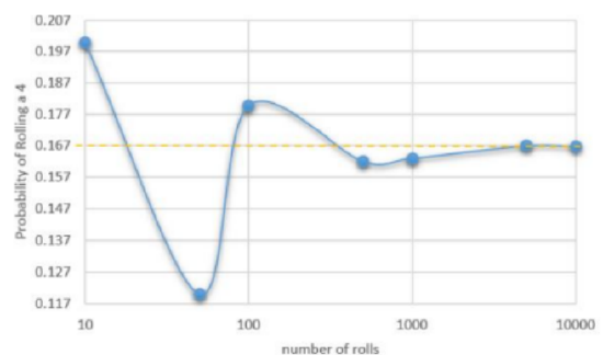
Figure \(\PageIndex{2}\)

You can compute experimental probabilities whenever it is not possible to calculate probabilities using other means. An example is if you want to find the probability that a family has 5 children, you would have to actually look at many families, and count how many have 5 children. Then you could calculate the probability. Another example is if you want to figure out if a die is fair. You would have to roll the die many times and count how often each side comes up. Make sure you repeat an experiment many times, because otherwise you will not be able to estimate the true probability of 5 children or the fairness of the die. This is due to the Law of Large Numbers, since the more times we repeat the experiment, the closer the experimental probabilities will get to the theoretical probabilities. For difficult theoretical probabilities, we can run computer simulations that can do an experiment repeatedly, many times, very quickly and come up with accurate estimates of the theoretical probability.

Example \(\PageIndex{5}\)

A fitness center coach kept track of members over the last year. They recorded if the person stretched before they exercised, and whether they sustained an injury. The following contingency table shows their results. Select one member at random and find the following probabilities.

	Injury	No Injury
Stretched	52	270
Did Not Stretch	21	57

1. Find the probability that a member sustained an injury.
2. Find the probability that a member did not stretch.
3. Find the probability that a member sustained an injury and did not stretch.

Solution

1. Find the totals for each row, column, and grand total.

	Injury	No Injury	Total
Stretched	52	270	322
Did Not Stretch	21	57	78
Total	73	327	400

Next, find the relative frequencies by dividing each number by the total of 400.

	Injury	No Injury	Total
Stretched	0.13	0.675	0.805
Did Not Stretch	0.0525	0.1425	0.195
Total	0.1825	0.8175	1

Using the formula for probability. we get P(Injury) = \(\dfrac{\text{Number of injuries}}{\text{Total number of people}}\) = \(\dfrac{73}{400}\) = 0.1825.

	Injury	No Injury	Total
Stretched	0.13	0.675	0.805
Did Not Stretch	0.0525	0.1425	0.195
Total	0.1825	0.8175	1

Using the table, we can get the same answer very quickly by just taking the column total under Injury to get 0.1825. As we get more complicated probability questions, these contingency tables will help organize your data.

2. Using the relative frequency contingency table, take the total of the row for all the members that did not stretch and we get the P(Did Not Stretch) = 0.195.

	Injury	No Injury	Total
Stretched	0.13	0.675	0.805
Did Not Stretch	0.0525	0.1425	0.195
Total	0.1825	0.8175	1

3. Using the relative frequency contingency table, take the intersection of the injury column with the did not stretch row and we get P(Injury and Did Not Stretch) = 0.0525.

	Injury	No Injury	Total
Stretched	0.13	0.675	0.805
Did Not Stretch	0.0525	0.1425	0.195
Total	0.1825	0.8175	1

Subjective Probability

Definition: Subjective Probability

Subjective probability is the probability of event A estimated using previous knowledge and is someone’s opinion.

Example \(\PageIndex{6}\)

Find the probability of meeting Dolly Parton.

Solution

I estimate the probability of meeting Dolly Parton to be \(1.2 \times 10^{-9}\) = 1.2 E-9 \(\approx\) 0.0000000012. This is a very small probability and essentially means that the probability is 0 and meeting Dolly Parton will not happen.

Example \(\PageIndex{7}\)

What is the probability it will rain tomorrow?

Solution

A weather reporter looks at several forecasts, uses their expert knowledge of the region, and reports the probability that it will rain tomorrow is 80%.