2.04 Using the Excel Spreadsheet provided to generate Descriptive Statistics

Last updated
Save as PDF

Page ID: 20125

\( \newcommand{\vecs}[1]{\overset { \scriptstyle \rightharpoonup} {\mathbf{#1}} } \) \( \newcommand{\vecd}[1]{\overset{-\!-\!\rightharpoonup}{\vphantom{a}\smash {#1}}} \)\(\newcommand{\id}{\mathrm{id}}\) \( \newcommand{\Span}{\mathrm{span}}\) \( \newcommand{\kernel}{\mathrm{null}\,}\) \( \newcommand{\range}{\mathrm{range}\,}\) \( \newcommand{\RealPart}{\mathrm{Re}}\) \( \newcommand{\ImaginaryPart}{\mathrm{Im}}\) \( \newcommand{\Argument}{\mathrm{Arg}}\) \( \newcommand{\norm}[1]{\| #1 \|}\) \( \newcommand{\inner}[2]{\langle #1, #2 \rangle}\) \( \newcommand{\Span}{\mathrm{span}}\) \(\newcommand{\id}{\mathrm{id}}\) \( \newcommand{\Span}{\mathrm{span}}\) \( \newcommand{\kernel}{\mathrm{null}\,}\) \( \newcommand{\range}{\mathrm{range}\,}\) \( \newcommand{\RealPart}{\mathrm{Re}}\) \( \newcommand{\ImaginaryPart}{\mathrm{Im}}\) \( \newcommand{\Argument}{\mathrm{Arg}}\) \( \newcommand{\norm}[1]{\| #1 \|}\) \( \newcommand{\inner}[2]{\langle #1, #2 \rangle}\) \( \newcommand{\Span}{\mathrm{span}}\)\(\newcommand{\AA}{\unicode[.8,0]{x212B}}\)

How to use the Excel Spreadsheet provided to generate descriptive statistics

On the Data and Descriptive Statistics tab, move to cell A1. You can type the numbers in the blue cells, and the spreadsheet will calculate the descriptive statistics. To use the Copy and Paste command, download the Excel spreadsheet DescriptiveStatistics.xlsx (click the link to download the Excel spreadsheet).

You will only be able to enter values in the blue cells.

Suppose your data is as follows.

635.7

509.5

500.3

735.3

575.1

463.4

477.3

642.8

492.8

642.4

772.7

659.5

502.1

Starting in cell A1 enter the data one point at a time.

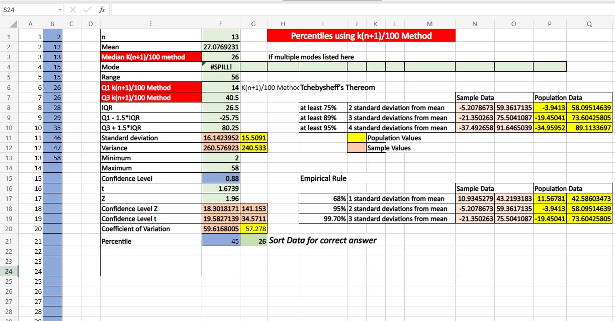
Once the data is entered into the Excel spreadsheet, the values are calculated for the following information. You can only enter values in the blue cells.

The sample size, n, is in cell E1.
The mean is in cell E2.
The median is in cell E3
The Mode is in cell E4
The range is in cell E5.
The first Quartile is in cell E6.
The third Quartile is in cell E7.
The interquartile range is in cell E8.
The low limit for outliers using Quartiles is in cell E9.
The upper limit for outlier using Quartile is in cell E10.
The standard deviation is in cell E11.
The variance is in cell E12.
The minimum is in cell E13.
The maximum is in cell E14.
The Coefficient of Variation is in cell E20 for sample data in F20 if the data represents all elements in the population.
The Empirical Rule Intervals are in cells M17 thru P19.
The Tchebysheff's Theorem's Intervals are in cells M8 thru P10.

The final Excel spreadsheet will display the following information.

Resulting Values
Sample Size	13
Mean	585.3
Median	575.1
Mode	No mode
Range	309.3
First Quartile Q1 (There are at least seven ways to compute this value)	500.3
Third Quartile Q3 (There are at least seven ways to compute this value)	642.8
Interquartile Range (Q3 - Q1)	142.5
Lower Limit for Outliers (Values below this value are considered outliers)	286.55
Upper Limit for Outliers (Values above this value are considered outliers)	856.55
Standard Deviation (Sample/Population)	103/98.9592
Variance (Sample/Population)	10609/9798.93
Minimum	463.4
Maximum	772.7
Coefficient of Variation (Sample/Population)	17.59781/16.90743
Empirical Rule (68% of data between) (Sample/Population)	[482.3, 688.3]/[486.3408, 684.2592]
Empirical Rule (95% of data between) (Sample/Population)	[379.3, 791.3]/[387.3816, 783.2184]
Empirical Rule (99.7% of data between) (Sample/Population)	[276.3, 894.3]/[288.4224, 882.1776]
Tchebysheff's Theorem (at least 75%) (Sample/Population)	[379.3, 791.3]/[387.3816, 783.2184]
Tchebysheff's Theorem (at least 89%) (Sample/Population)	[276.3, 894.3]/[288.4224, 882.1776]
Tchebysheff's Theorem (at least 95%) (Sample/Population)	[173.3, 997.3]/[189.4632, 981.1368]

Using the (n+1) method to compute the Quartiles using the k^th Percentile

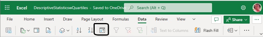
To find the Quartiles using the method outlined in the Introductory Business Statistic book. Copy the data on the Data and Descriptive Statistics spreadsheet and Paste 123 the data on the Quartile calculation spreadsheet starting at cell A1. Then highlight the data and hit the Data tab and click the Sort icon .

The dialog box below will appear. Click on Just sort button.

The dialog box will appear. Click on the Just sort button. Then un-select the My data has headers box and click the OK button.

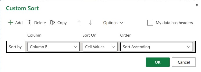
The data will be sorted. Then hit the F9 key to recalculate the values.

Q1 the first quartile is equal to 25(13+1)/100 = 3.5. Since 3.5 is not an integer take the 3rd and 4th value and average them (13+15)/2 = 14. Q₁ = 14.

Median is the second quartile is equal to 50(13+1)/100 = 7. Since 7 is an integer, the median is the 7th value, 26.

Q3, the third quartile is 75(13+1)/100 = 10.5. Since 10.5 is not an integer, the third quartile is the average of the 11^th and 12^th value, (35+46)/2 = 40.5.