
2.5: Measures of Central Tendency
- Page ID
- 41768
\( \newcommand{\vecs}[1]{\overset { \scriptstyle \rightharpoonup} {\mathbf{#1}} } \)
\( \newcommand{\vecd}[1]{\overset{-\!-\!\rightharpoonup}{\vphantom{a}\smash {#1}}} \)
\( \newcommand{\dsum}{\displaystyle\sum\limits} \)
\( \newcommand{\dint}{\displaystyle\int\limits} \)
\( \newcommand{\dlim}{\displaystyle\lim\limits} \)
\( \newcommand{\id}{\mathrm{id}}\) \( \newcommand{\Span}{\mathrm{span}}\)
( \newcommand{\kernel}{\mathrm{null}\,}\) \( \newcommand{\range}{\mathrm{range}\,}\)
\( \newcommand{\RealPart}{\mathrm{Re}}\) \( \newcommand{\ImaginaryPart}{\mathrm{Im}}\)
\( \newcommand{\Argument}{\mathrm{Arg}}\) \( \newcommand{\norm}[1]{\| #1 \|}\)
\( \newcommand{\inner}[2]{\langle #1, #2 \rangle}\)
\( \newcommand{\Span}{\mathrm{span}}\)
\( \newcommand{\id}{\mathrm{id}}\)
\( \newcommand{\Span}{\mathrm{span}}\)
\( \newcommand{\kernel}{\mathrm{null}\,}\)
\( \newcommand{\range}{\mathrm{range}\,}\)
\( \newcommand{\RealPart}{\mathrm{Re}}\)
\( \newcommand{\ImaginaryPart}{\mathrm{Im}}\)
\( \newcommand{\Argument}{\mathrm{Arg}}\)
\( \newcommand{\norm}[1]{\| #1 \|}\)
\( \newcommand{\inner}[2]{\langle #1, #2 \rangle}\)
\( \newcommand{\Span}{\mathrm{span}}\) \( \newcommand{\AA}{\unicode[.8,0]{x212B}}\)
\( \newcommand{\vectorA}[1]{\vec{#1}} % arrow\)
\( \newcommand{\vectorAt}[1]{\vec{\text{#1}}} % arrow\)
\( \newcommand{\vectorB}[1]{\overset { \scriptstyle \rightharpoonup} {\mathbf{#1}} } \)
\( \newcommand{\vectorC}[1]{\textbf{#1}} \)
\( \newcommand{\vectorD}[1]{\overrightarrow{#1}} \)
\( \newcommand{\vectorDt}[1]{\overrightarrow{\text{#1}}} \)
\( \newcommand{\vectE}[1]{\overset{-\!-\!\rightharpoonup}{\vphantom{a}\smash{\mathbf {#1}}}} \)
\( \newcommand{\vecs}[1]{\overset { \scriptstyle \rightharpoonup} {\mathbf{#1}} } \)
\(\newcommand{\longvect}{\overrightarrow}\)
\( \newcommand{\vecd}[1]{\overset{-\!-\!\rightharpoonup}{\vphantom{a}\smash {#1}}} \)
\(\newcommand{\avec}{\mathbf a}\) \(\newcommand{\bvec}{\mathbf b}\) \(\newcommand{\cvec}{\mathbf c}\) \(\newcommand{\dvec}{\mathbf d}\) \(\newcommand{\dtil}{\widetilde{\mathbf d}}\) \(\newcommand{\evec}{\mathbf e}\) \(\newcommand{\fvec}{\mathbf f}\) \(\newcommand{\nvec}{\mathbf n}\) \(\newcommand{\pvec}{\mathbf p}\) \(\newcommand{\qvec}{\mathbf q}\) \(\newcommand{\svec}{\mathbf s}\) \(\newcommand{\tvec}{\mathbf t}\) \(\newcommand{\uvec}{\mathbf u}\) \(\newcommand{\vvec}{\mathbf v}\) \(\newcommand{\wvec}{\mathbf w}\) \(\newcommand{\xvec}{\mathbf x}\) \(\newcommand{\yvec}{\mathbf y}\) \(\newcommand{\zvec}{\mathbf z}\) \(\newcommand{\rvec}{\mathbf r}\) \(\newcommand{\mvec}{\mathbf m}\) \(\newcommand{\zerovec}{\mathbf 0}\) \(\newcommand{\onevec}{\mathbf 1}\) \(\newcommand{\real}{\mathbb R}\) \(\newcommand{\twovec}[2]{\left[\begin{array}{r}#1 \\ #2 \end{array}\right]}\) \(\newcommand{\ctwovec}[2]{\left[\begin{array}{c}#1 \\ #2 \end{array}\right]}\) \(\newcommand{\threevec}[3]{\left[\begin{array}{r}#1 \\ #2 \\ #3 \end{array}\right]}\) \(\newcommand{\cthreevec}[3]{\left[\begin{array}{c}#1 \\ #2 \\ #3 \end{array}\right]}\) \(\newcommand{\fourvec}[4]{\left[\begin{array}{r}#1 \\ #2 \\ #3 \\ #4 \end{array}\right]}\) \(\newcommand{\cfourvec}[4]{\left[\begin{array}{c}#1 \\ #2 \\ #3 \\ #4 \end{array}\right]}\) \(\newcommand{\fivevec}[5]{\left[\begin{array}{r}#1 \\ #2 \\ #3 \\ #4 \\ #5 \\ \end{array}\right]}\) \(\newcommand{\cfivevec}[5]{\left[\begin{array}{c}#1 \\ #2 \\ #3 \\ #4 \\ #5 \\ \end{array}\right]}\) \(\newcommand{\mattwo}[4]{\left[\begin{array}{rr}#1 \amp #2 \\ #3 \amp #4 \\ \end{array}\right]}\) \(\newcommand{\laspan}[1]{\text{Span}\{#1\}}\) \(\newcommand{\bcal}{\cal B}\) \(\newcommand{\ccal}{\cal C}\) \(\newcommand{\scal}{\cal S}\) \(\newcommand{\wcal}{\cal W}\) \(\newcommand{\ecal}{\cal E}\) \(\newcommand{\coords}[2]{\left\{#1\right\}_{#2}}\) \(\newcommand{\gray}[1]{\color{gray}{#1}}\) \(\newcommand{\lgray}[1]{\color{lightgray}{#1}}\) \(\newcommand{\rank}{\operatorname{rank}}\) \(\newcommand{\row}{\text{Row}}\) \(\newcommand{\col}{\text{Col}}\) \(\renewcommand{\row}{\text{Row}}\) \(\newcommand{\nul}{\text{Nul}}\) \(\newcommand{\var}{\text{Var}}\) \(\newcommand{\corr}{\text{corr}}\) \(\newcommand{\len}[1]{\left|#1\right|}\) \(\newcommand{\bbar}{\overline{\bvec}}\) \(\newcommand{\bhat}{\widehat{\bvec}}\) \(\newcommand{\bperp}{\bvec^\perp}\) \(\newcommand{\xhat}{\widehat{\xvec}}\) \(\newcommand{\vhat}{\widehat{\vvec}}\) \(\newcommand{\uhat}{\widehat{\uvec}}\) \(\newcommand{\what}{\widehat{\wvec}}\) \(\newcommand{\Sighat}{\widehat{\Sigma}}\) \(\newcommand{\lt}{<}\) \(\newcommand{\gt}{>}\) \(\newcommand{\amp}{&}\) \(\definecolor{fillinmathshade}{gray}{0.9}\)- Discuss common measures of central tendency: mean, median, and mode
- Introduce the trimmed mean
Section \(2.5\) Excel File (contains all of the data sets for this section)
Introduction to Measures of Central Tendency
We understand data by looking at distributions (graphs and tables) and box-and-whisker plots. With relative frequency distributions, we determined classes and then computed the percentage of observations in each class. With box-and-whisker plots, we determined four classes each with \(25\%\) of the observations. These were constructed using descriptive statistics and allowed us to see where and how the data values fell; we could see the distribution of the data. In this section, we discuss descriptive statistics that indicate the center of the data. There are many different ways to define the center of a data set; each measure has strengths and weaknesses. We discuss the three most common measures of central tendency: mode, median, and mean.
Mode
When examining a frequency distribution, either a table or a graph, our attention often gravitates to the highest frequency: the value that occurs the most. Sometimes, this highest frequency occurs in multiple classes. We call the class(es) with the highest frequency the mode(s). If there is only one class with the highest frequency, we call the distribution unimodal; otherwise, we call it multimodal. The mode is a measure of central tendency by describing the classes that occur most frequently; the distribution is often centered around these most common values. The mode can be computed for any variable regardless of its level of measurement. It is the only measure we will discuss that is defined for nominal data.
Recall the frequency distribution of colors of candies in a bag of M&M's from our previous discussion.
| Color | Frequency | Relative Frequency |
|---|---|---|
| Brown | \(17\) | \(\frac{17}{55}\approx0.309\) |
| Red | \(18\) | \(\frac{18}{55}\approx0.327\) |
| Yellow | \(7\) | \(\frac{7}{55}\approx0.127\) |
| Green | \(7\) | \(\frac{7}{55}\approx0.127\) |
| Blue | \(2\) | \(\frac{2}{55}\approx0.036\) |
| Orange | \(4\) | \(\frac{4}{55}\approx0.073\) |
1. Show that this data set is unimodal and give the mode.
- Answer
-
The mode is the value (characteristic) that appears most frequently. Red is the only mode since red appears \(18\) times, and all other colors appear fewer than that. Note that yellow and green are not modes even though \(7\) appears twice.
2. Show the set of colors could be multimodal after consuming one candy.
- Answer
-
We would have to reduce the number of red candies to make the set multimodal. If we eat one red candy, we would have \(17\) brown and \(17\) red candies. Since every other color appears fewer than \(17\) times, we have two modes: red and brown. The set would be multimodal, specifically bimodal (since there are two modes).
3. What is the minimum number of candies one would have to eat for orange to be the only mode?
- Answer
-
Since there are only \(4\) orange candies, we would have to reduce the number of every other color to less than \(4.\) If we ate \(14\) brown, \(15\) red, \(4\) yellow, and \(4\) green candies, we would have \(3\) of each of those colors, \(2\) blues, and \(4\) orange making orange the mode. We need to eat, at minimum, \(14+\)\(15+\)\(4+\)\(4\) \(=37\) candies. YUM!
It is easy to see the possible issues with the mode as a measure of central tendency. Consider the following data set: \(1,\) \(2,\) \(3,\) \(4,\) \(5,\) \(6,\) \(7,\) \(8,\) \(9,\) \(10,\) \(11,\) \(1000,\) \(1000.\) The mode is \(1000,\) but is that a reasonable value for the center of this data? The use of the mode is often minimal with quantitative data.
Median
When constructing a box-and-whisker plot, we computed five measures: minimum, first quartile, second quartile, third quartile, and maximum. Each of these measures relative position and relies on ordering the data. A natural measure of central tendency would be a value that splits the data evenly below and above, such as the second quartile, the \(50^{th}\) percentile. We generally refer to it as the median, one of the most common measures of central tendency. Since the median requires an ordering from smallest to greatest, it cannot be computed for nominal variables, but it can be calculated for ordinal, interval, and ratio variables.
Arithmetic Mean
The third measure, called the arithmetic mean, is arguably the most common measure of central tendency. Bar graphs may remind us of geometric figures placed along a scale, making us wonder: what is the center of mass? This would be the point at which the figure would balance if it were propped up only at that point. How might we find such a point? Consider Figure \(\PageIndex{1}\) and the location of the fulcrum. Why is it where it is?
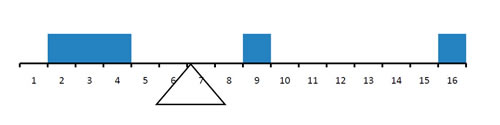
Figure \(\PageIndex{1}\): A simple distribution balanced upon its center of mass
Note that there are more blocks to the left of the fulcrum than to the right, but the figure is still balanced. The blocks on the left are closer to the fulcrum than the far block on the right. The distance a block is away from the fulcrum must play a part in this balancing act. Imagine keeping the fulcrum fixed and removing the blocks on the left side. What happens to the system? The blocks on the right with the absence of the blocks on the left will rotate clockwise. On the other hand, imagine keeping the fulcrum fixed and removing the blocks on the right side. We again get motion, but this time in the counterclockwise direction. These natural intuitions, hopefully fueled by your childhood playground experiences, form the basis for figuring out where the fulcrum needs to be placed in order to balance the system. As we progress, this balancing point is the arithmetic mean.
Since each observation is equally important, we consider each observation (block) having the same weight \(w\) distributed evenly across a uniform-sized block, and then we simply stack the blocks on our scale with the blocks centered on their value. Note that there is only one location \(c\) that our distribution balances. When it is balanced, there is no motion. The rotational force from the blocks to the right of \(c,\) eliciting a clockwise motion, is equal to the rotational force from the blocks to the left of \(c,\) eliciting a counterclockwise motion. Note, as partially intuited above, the rotational force from each block is equal to the distance the block is from \(c\) multiplied by the weight of the block. And finally, the total rotational force is equal to the sum of the rotational forces from the individual blocks. This yields the following equation:\[\underbrace{(c-2)w}_{1^{st}\text{ block}}+\underbrace{(c-3)w}_{2^{nd} \text{ block} }+\underbrace{(c-4)w}_{3^{rd} \text{ block} }=\underbrace{(9-c)w}_{4^{th} \text{ block} }+\underbrace{(16-c)w}_{5^{th} \text{ block} }\nonumber.\]Note that every term has the same weight, \(w,\) which cancels algebraically. Move all of the \(c\) terms together and constants together to produce the equivalent equation \[5c=2+3+4+9+16\nonumber\]\[c=\frac{2+3+4+9+16}{5}=\frac{34}{5}\nonumber\]
- Optional general derivation for the mathematically inclined
-
We could have chosen to factor out a negative sign from the left side to yield:\[-((2-c)+(3-c)+(4-c))=(9-c)+(16-c)\nonumber\]Meaning that our equation is equivalent to \[0=(2-c)+(3-c)+(4-c)+(9-c)+(16-c)\nonumber\]
We may generalize. Let \(x_i\) represent our \(i^{th}\) value from our collection of \(n\) data values. To find our center of mass \(c,\) we need the rotational forces to balance, which is equivalent to the following:\[0=\sum_{i=1}^n (x_i-c)=x_1-c+x_2-c+...x_n-c= \left( {\sum_{i=1}^n x_i} \right) - n \cdot c \nonumber\]Meaning \[c=\dfrac{1}{n}\sum_{i=1}^n x_i\nonumber\]
This is the familiar formula for the arithmetic mean, what many call "average." The arithmetic mean of a data set is the center of mass for its frequency distribution and is a measure of central tendency.
The arithmetic mean plays a significant role in statistics and throughout this course. There are several different types of means, but given the prevalence of the arithmetic mean, we will refer to the arithmetic mean simply as the mean. We have standard notation to differentiate the mean as a statistic, denoted \(\bar{x},\) from the mean as a parameter, denoted \(\mu.\) This latter symbol is the lowercase Greek letter mu. Recall that parameters are generally denoted with Greek letters and refer to properties of a population, not a sample. Notice the similarity in the formulas for computations below:\[\bar{x}=\dfrac{\sum x_i}{n} ~~~~~~~~~\mu=\dfrac{\sum x_i}{N}\nonumber\]Note: the summations used in these formulas do not include any indexing information. When this is the case, sum over all observations.
Since the arithmetic mean requires that the differences between values have meaning, it cannot be computed for nominal or ordinal variables but can be computed for interval and ratio-level data.
Consider the following distributions. Determine which of the common measures of central tendency are indicated by the blue and pink bars below the scaling axis. Explain your reasoning.


Figure \(\PageIndex{2}\): A symmetric distribution (left) and a positively skewed distribution (right)
- Answer
-
There are three standard measures of central tendency: mode, median, and mean. The distribution on the left is unimodal and symmetric. The distribution on the right is also unimodal but is positively skewed. The mean, median, and mode are all equal in the left distribution. This follows from the fact that it is unimodal and symmetric. (Can you explain why?) The mode of the right distribution is less than both colored bars on the scale axis; thus, the bars do not represent the mode.
Determining which bar represents the mean is a little more complicated. Recall that the number of observations above the median and below the median should be equal. The median splits the number of observations in half, but it is difficult to tell which bar has the same number of observations on both sides. When analyzing relationships, it is best to alter only one variable at a time. If we increase the maximum value (move it to the right), the median won't change. However, the mean would become larger to keep the figure balanced. A positive skew moves the mean to the right, and the mean is larger than the median. The blue bar is the mean, and the pink bar is the median.
In the previous exercise, we decided that the mean would be a larger value than the median in a positively skewed data set. A similar argument yields that the mean takes on smaller values than the median in negatively skewed data. This is because the mean incorporates every value into its computation, while the median only cares about the relative position of the values. We recommend computing the median as the better measure of center when the data is skewed or has values of a more extreme magnitude than the rest.
Determine which measures of central tendency are appropriate. Which would be the most appropriate? Explain.
1. Evaluations rated on a scale of \(1\) through \(5\)
- Answer
-
Rating scales are measured on the ordinal scale. While statisticians debate the legitimacy of averaging ordinal data, we recommend avoiding the practice. Median and mode are eligible candidates. The median is used more frequently than the mode; it is our measure of choice.
2. Salaries
- Answer
-
Salaries are measured on the ratio scale making mode, median, and mean eligible candidates. However, salary data is often positively skewed, making the median a better choice.
3. Heights
- Answer
-
Heights are measured on the ratio scale. Again, the mode, median, and mean are eligible candidates. Heights are not generally highly skewed, making the mean a better choice.
4. Shirt sizes
- Answer
-
Shirt sizes are measured on the ordinal scale. Between mode and median, we would choose the median
5. Favorite candies
- Answer
-
Favorite candies are measured on the nominal scale. The only option is mode.
Create a data set consisting of \(10\) observations such that the mean is \(15\), the median is \(14\), and the mode is \(17\).
- Answer
-
Use the Section \(2.5\) Excel file to check your solution by typing your \(10\) values in the second column. The cells with the running calculations will turn green when that aspect of the data set is correct. There are infinitely many possible data sets. Do not fret if your solution is different than your classmates' solutions.
Sometimes, working backward can be difficult. First, consider what each measure says about the data. If the mean is \(15\) with \(10\) observations, the sum of all the values needs to be \(150\). If the median is \(14\), the average of the \(5^{th}\) and \(6^{th}\) values in rank order, must be \(14\). If the mode is \(17\), \(17\) must appear the most number of times (at least twice, if every other number only appears once). Start with the most restrictive measures and work through them all. We recommend starting with the median, then the mode, and ending with the mean.
Trimmed Mean
When data is skewed or has values more extreme than the rest, we recommended using the median as a measure of central tendency. There is a less common measure, a hybrid between the mean and median, that can also be used. It is called the trimmed mean; its definition differs across the literature, but its underlying idea is consistent. When we have data of this type, the observations that significantly affect the mean value are the extreme values of the data. To mitigate their influence, we trim a certain percentage of the observations from both the top and the bottom and compute the mean on the remaining data.
When running across the trimmed mean in literature or research, check what definition is being used, as there are subtle differences that are good to be aware of. We now provide our working definition of the \(p\%\)-trimmed mean. Trim \(p\%\) of the data from the top and \(p\%\) of the data from the bottom for a total of \(2p\%\) and then compute the mean of the remaining data. If \(p\%\) is not a whole number, remove the smallest number of observations such that at least \(p\%\) of the observations are removed.
Compute the mode, median, mean, and \(10\%\)-trimmed mean for the following sample data.
{\(10, 6, 5, 25, 10, 11, 17, 13, 15, 13, 19, 10\)}
- Answer
-
Ordering and counting the data for the median and \(10\%\)-trimmed mean is necessary.
{\(5, 6, 10, 10, 10, 11, 13, 13, 15, 17, 19, 25\)} with \(n=12\)
Mode: \(10\) occurs most frequently with three occurrences. \(13\) comes in at second with two occurrences. The mode is \(10.\)
Median: We must first compute our rank \(R=\frac{50}{100}(12)\) \(=6.\) Since it is a natural number, we look at the \(6^{th}\) and \(7^{th}\) values, \(11\) and \(13\) respectively. Our median is the midpoint, \(\frac{1}{2}(11+13)\) \(=12\)
Mean: \(\bar{x}\) \(=\frac{5+6+10+10+10+11+13+13+15+17+19+25}{12}\) \(=\frac{154}{12}\) \(=12\frac{5}{6}\) \(=12.8\overline{3}\)
\(10\%\)-trimmed mean: We must first compute how many observations we must remove. \(10\%\) of \(12\) is \(1.2.\) This is not a whole number; we, therefore, remove two observations from the bottom and two from the top. We find the average of the following set:
{\(10, 10, 10, 11, 13, 13, 15, 17\)}
\(10\%\)-trimmed mean\(=\frac{10+10+10+11+13+13+15+17}{8}\) \(=\frac{99}{8}\) \(=12\frac{3}{8}\) \(=12.375\)
Notice we get an incorrect value for the trimmed mean unless we first sort the data.