
Ch 12.2 and 12.4 Scatter Plot and Correlation
- Page ID
- 15927
\( \newcommand{\vecs}[1]{\overset { \scriptstyle \rightharpoonup} {\mathbf{#1}} } \)
\( \newcommand{\vecd}[1]{\overset{-\!-\!\rightharpoonup}{\vphantom{a}\smash {#1}}} \)
\( \newcommand{\id}{\mathrm{id}}\) \( \newcommand{\Span}{\mathrm{span}}\)
( \newcommand{\kernel}{\mathrm{null}\,}\) \( \newcommand{\range}{\mathrm{range}\,}\)
\( \newcommand{\RealPart}{\mathrm{Re}}\) \( \newcommand{\ImaginaryPart}{\mathrm{Im}}\)
\( \newcommand{\Argument}{\mathrm{Arg}}\) \( \newcommand{\norm}[1]{\| #1 \|}\)
\( \newcommand{\inner}[2]{\langle #1, #2 \rangle}\)
\( \newcommand{\Span}{\mathrm{span}}\)
\( \newcommand{\id}{\mathrm{id}}\)
\( \newcommand{\Span}{\mathrm{span}}\)
\( \newcommand{\kernel}{\mathrm{null}\,}\)
\( \newcommand{\range}{\mathrm{range}\,}\)
\( \newcommand{\RealPart}{\mathrm{Re}}\)
\( \newcommand{\ImaginaryPart}{\mathrm{Im}}\)
\( \newcommand{\Argument}{\mathrm{Arg}}\)
\( \newcommand{\norm}[1]{\| #1 \|}\)
\( \newcommand{\inner}[2]{\langle #1, #2 \rangle}\)
\( \newcommand{\Span}{\mathrm{span}}\) \( \newcommand{\AA}{\unicode[.8,0]{x212B}}\)
\( \newcommand{\vectorA}[1]{\vec{#1}} % arrow\)
\( \newcommand{\vectorAt}[1]{\vec{\text{#1}}} % arrow\)
\( \newcommand{\vectorB}[1]{\overset { \scriptstyle \rightharpoonup} {\mathbf{#1}} } \)
\( \newcommand{\vectorC}[1]{\textbf{#1}} \)
\( \newcommand{\vectorD}[1]{\overrightarrow{#1}} \)
\( \newcommand{\vectorDt}[1]{\overrightarrow{\text{#1}}} \)
\( \newcommand{\vectE}[1]{\overset{-\!-\!\rightharpoonup}{\vphantom{a}\smash{\mathbf {#1}}}} \)
\( \newcommand{\vecs}[1]{\overset { \scriptstyle \rightharpoonup} {\mathbf{#1}} } \)
\( \newcommand{\vecd}[1]{\overset{-\!-\!\rightharpoonup}{\vphantom{a}\smash {#1}}} \)
\(\newcommand{\avec}{\mathbf a}\) \(\newcommand{\bvec}{\mathbf b}\) \(\newcommand{\cvec}{\mathbf c}\) \(\newcommand{\dvec}{\mathbf d}\) \(\newcommand{\dtil}{\widetilde{\mathbf d}}\) \(\newcommand{\evec}{\mathbf e}\) \(\newcommand{\fvec}{\mathbf f}\) \(\newcommand{\nvec}{\mathbf n}\) \(\newcommand{\pvec}{\mathbf p}\) \(\newcommand{\qvec}{\mathbf q}\) \(\newcommand{\svec}{\mathbf s}\) \(\newcommand{\tvec}{\mathbf t}\) \(\newcommand{\uvec}{\mathbf u}\) \(\newcommand{\vvec}{\mathbf v}\) \(\newcommand{\wvec}{\mathbf w}\) \(\newcommand{\xvec}{\mathbf x}\) \(\newcommand{\yvec}{\mathbf y}\) \(\newcommand{\zvec}{\mathbf z}\) \(\newcommand{\rvec}{\mathbf r}\) \(\newcommand{\mvec}{\mathbf m}\) \(\newcommand{\zerovec}{\mathbf 0}\) \(\newcommand{\onevec}{\mathbf 1}\) \(\newcommand{\real}{\mathbb R}\) \(\newcommand{\twovec}[2]{\left[\begin{array}{r}#1 \\ #2 \end{array}\right]}\) \(\newcommand{\ctwovec}[2]{\left[\begin{array}{c}#1 \\ #2 \end{array}\right]}\) \(\newcommand{\threevec}[3]{\left[\begin{array}{r}#1 \\ #2 \\ #3 \end{array}\right]}\) \(\newcommand{\cthreevec}[3]{\left[\begin{array}{c}#1 \\ #2 \\ #3 \end{array}\right]}\) \(\newcommand{\fourvec}[4]{\left[\begin{array}{r}#1 \\ #2 \\ #3 \\ #4 \end{array}\right]}\) \(\newcommand{\cfourvec}[4]{\left[\begin{array}{c}#1 \\ #2 \\ #3 \\ #4 \end{array}\right]}\) \(\newcommand{\fivevec}[5]{\left[\begin{array}{r}#1 \\ #2 \\ #3 \\ #4 \\ #5 \\ \end{array}\right]}\) \(\newcommand{\cfivevec}[5]{\left[\begin{array}{c}#1 \\ #2 \\ #3 \\ #4 \\ #5 \\ \end{array}\right]}\) \(\newcommand{\mattwo}[4]{\left[\begin{array}{rr}#1 \amp #2 \\ #3 \amp #4 \\ \end{array}\right]}\) \(\newcommand{\laspan}[1]{\text{Span}\{#1\}}\) \(\newcommand{\bcal}{\cal B}\) \(\newcommand{\ccal}{\cal C}\) \(\newcommand{\scal}{\cal S}\) \(\newcommand{\wcal}{\cal W}\) \(\newcommand{\ecal}{\cal E}\) \(\newcommand{\coords}[2]{\left\{#1\right\}_{#2}}\) \(\newcommand{\gray}[1]{\color{gray}{#1}}\) \(\newcommand{\lgray}[1]{\color{lightgray}{#1}}\) \(\newcommand{\rank}{\operatorname{rank}}\) \(\newcommand{\row}{\text{Row}}\) \(\newcommand{\col}{\text{Col}}\) \(\renewcommand{\row}{\text{Row}}\) \(\newcommand{\nul}{\text{Nul}}\) \(\newcommand{\var}{\text{Var}}\) \(\newcommand{\corr}{\text{corr}}\) \(\newcommand{\len}[1]{\left|#1\right|}\) \(\newcommand{\bbar}{\overline{\bvec}}\) \(\newcommand{\bhat}{\widehat{\bvec}}\) \(\newcommand{\bperp}{\bvec^\perp}\) \(\newcommand{\xhat}{\widehat{\xvec}}\) \(\newcommand{\vhat}{\widehat{\vvec}}\) \(\newcommand{\uhat}{\widehat{\uvec}}\) \(\newcommand{\what}{\widehat{\wvec}}\) \(\newcommand{\Sighat}{\widehat{\Sigma}}\) \(\newcommand{\lt}{<}\) \(\newcommand{\gt}{>}\) \(\newcommand{\amp}{&}\) \(\definecolor{fillinmathshade}{gray}{0.9}\)Ch 12.2 and 12.4 Scatter plot and correlation
Correlation
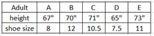
Ex1. Given the matched pair sample data below. Can we conclude correlation between height and shoe size?

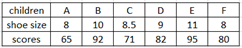
Ex2. Given the matched pair sample below, can we conclude correlation between shoe size and math scores?

Terms:
Correlation: Correlation between matched pair data (x, y) exists when values of y are associated with the values of x. Note: correlation does not imply causation.
Tools to study correlation:
1) Graphical: scatter plot. Each pair of (x, y) is plotted as one point on a graph. If a systematic pattern exists, there is correlation between x and y. Note: the pattern can be linear or non-linear.
2) Mathematical: use (x, y) sample data to calculate a correlation coefficient (r) . Value of r is used to determine if linear correlation exists and the strength and type of linear correlation.
Scatter plot examples
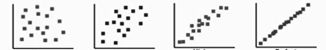
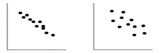


no correlation weak positive strong positive prefect positive strong negative weak negative non-linear correlations
Scatter plot
Construct scatter plot: Enter x and y data to statdisk in two different columns. Data/scatter plot/
Select x and y columns. Uncheck show regression line.
copy the scatter plot by labeling the axis and axis title.
Correlation coefficient (r )
The value shows how strongly the matched pair data x, y related to each other linearly.
Use Statdisk, enter data to 2 different columns.
Analysis/Correlation and Regression. Enter significance, select x and y columns, Evaluate.
output under “correlation result”
r = is the correlation coefficient, critical r is the critical threshold for evidence of linear correlation.
p-value is the probability of getting the sample under the H0 assumption of no linear correlation.
Properties of r:
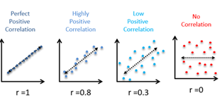
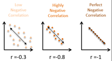
1) between -1 and 1. r = 0 means no linear correlation. r =1 means perfect linear correlation.
2) If |r| is close to 1, there is strong linear correlation. If |r| is close to 0, there is weak linear correlation.
3) r > 0, correlation is positive, x increase, y increase.
r < 0, correlation is negative, x increase, y decrease.
Relationship between scatter plot and correlation coefficient r.
Use Guess correlation game to understand relationship between r and scatter plot. https://istics.net/Correlations/
To determine if matched pair (x, y) has linear correlation:
Step 1: Check scatter plot, If non -linear pattern exists, conclude no linear correlation.
Step 2:
Method 1: Use Hypothesis test method with a given α.
ρ = correlation coefficient for population.
r = correlation coefficient for sample.
H0: ρ = 0 (no linear correlation) Ha: : ρ ≠ 0
Use statdisk/Analysis/Correlation and Regression/ to find p-value.
P-value ≤ α Reject H0, conclude linear correlation
p-value > α Fail to reject H0, conclude no linear correlation.
Method2: Compare r and critical value.
Use Analysis/Correlation and Regression to find r and critical r.
If – critical r ≤ r ≤ +critical r , conclude no linear correlation.
If r < - critical r or r > + critical value of n and α, conclude linear correlation.
Note: Check scatter plot for non-linear correlation before deciding linear correlation. Do not depend on r only or p-value only.
Ex1. Determine if linear correlation exists between the following pairs of r and p-value given n and α. Assume scatter plots do not show any non-linear patterns.
a) r = – 0.823, critical r = ±754
Since r is < - 754, conclude there is linear correlation.
b) α = 0.05, p-value = 0.012
Since only p-value is given, use hypothesis testing method
0.012 < 0.05, Reject H0, conclude there is linear correlation.
Ex2. Determine if linear correlation exists between height and shoe size in the given matched pair data. Use α= 0.05
Enter data Statdisk data columns. Statdisk/data/scatter plot/uncheck regression line.
 Graph does not show non-linear pattern.
Analysis/Correlation and Regression/
Select height and shoe size columns.
Output: r = 0.8485, critical r = ±0.8783, p-value = 0.0692
Method 1: (p-value method)
0.0691 > 0.05, fail to reject H0, conclude no linear correlation.
Method 2: (critical value method)
0.8485 < 0.878, conclude no linear correlation.
Ex3. Determine if linear correlation exists between shoe size and math scores for 6 children. use α = 0.05
Enter to statdisk data columns.
 Data/scatter plot/ select data columns, uncheck show regression line.
Scatter plot does not show non-linear pattern.
Analysis/Correlation and Regression/enter significance.
Select data columns. Evaluate
Output: r = 0.8758, critical r =±0.8114, p-value = 0.0222
Method 1: (p-value method)
p-value 0.0222 < 0.05 Reject H0, conclude linear correlation.
Method 2: (critical value method)
0.876 > 0.811, conclude linear correlation
Other properties of r:
1) r does not change if x and y switches.
2) r does not change when different units are used in x and/or y.