6.3: Using the Normal Distribution
- Page ID
- 20046
\( \newcommand{\vecs}[1]{\overset { \scriptstyle \rightharpoonup} {\mathbf{#1}} } \)
\( \newcommand{\vecd}[1]{\overset{-\!-\!\rightharpoonup}{\vphantom{a}\smash {#1}}} \)
\( \newcommand{\dsum}{\displaystyle\sum\limits} \)
\( \newcommand{\dint}{\displaystyle\int\limits} \)
\( \newcommand{\dlim}{\displaystyle\lim\limits} \)
\( \newcommand{\id}{\mathrm{id}}\) \( \newcommand{\Span}{\mathrm{span}}\)
( \newcommand{\kernel}{\mathrm{null}\,}\) \( \newcommand{\range}{\mathrm{range}\,}\)
\( \newcommand{\RealPart}{\mathrm{Re}}\) \( \newcommand{\ImaginaryPart}{\mathrm{Im}}\)
\( \newcommand{\Argument}{\mathrm{Arg}}\) \( \newcommand{\norm}[1]{\| #1 \|}\)
\( \newcommand{\inner}[2]{\langle #1, #2 \rangle}\)
\( \newcommand{\Span}{\mathrm{span}}\)
\( \newcommand{\id}{\mathrm{id}}\)
\( \newcommand{\Span}{\mathrm{span}}\)
\( \newcommand{\kernel}{\mathrm{null}\,}\)
\( \newcommand{\range}{\mathrm{range}\,}\)
\( \newcommand{\RealPart}{\mathrm{Re}}\)
\( \newcommand{\ImaginaryPart}{\mathrm{Im}}\)
\( \newcommand{\Argument}{\mathrm{Arg}}\)
\( \newcommand{\norm}[1]{\| #1 \|}\)
\( \newcommand{\inner}[2]{\langle #1, #2 \rangle}\)
\( \newcommand{\Span}{\mathrm{span}}\) \( \newcommand{\AA}{\unicode[.8,0]{x212B}}\)
\( \newcommand{\vectorA}[1]{\vec{#1}} % arrow\)
\( \newcommand{\vectorAt}[1]{\vec{\text{#1}}} % arrow\)
\( \newcommand{\vectorB}[1]{\overset { \scriptstyle \rightharpoonup} {\mathbf{#1}} } \)
\( \newcommand{\vectorC}[1]{\textbf{#1}} \)
\( \newcommand{\vectorD}[1]{\overrightarrow{#1}} \)
\( \newcommand{\vectorDt}[1]{\overrightarrow{\text{#1}}} \)
\( \newcommand{\vectE}[1]{\overset{-\!-\!\rightharpoonup}{\vphantom{a}\smash{\mathbf {#1}}}} \)
\( \newcommand{\vecs}[1]{\overset { \scriptstyle \rightharpoonup} {\mathbf{#1}} } \)
\(\newcommand{\longvect}{\overrightarrow}\)
\( \newcommand{\vecd}[1]{\overset{-\!-\!\rightharpoonup}{\vphantom{a}\smash {#1}}} \)
\(\newcommand{\avec}{\mathbf a}\) \(\newcommand{\bvec}{\mathbf b}\) \(\newcommand{\cvec}{\mathbf c}\) \(\newcommand{\dvec}{\mathbf d}\) \(\newcommand{\dtil}{\widetilde{\mathbf d}}\) \(\newcommand{\evec}{\mathbf e}\) \(\newcommand{\fvec}{\mathbf f}\) \(\newcommand{\nvec}{\mathbf n}\) \(\newcommand{\pvec}{\mathbf p}\) \(\newcommand{\qvec}{\mathbf q}\) \(\newcommand{\svec}{\mathbf s}\) \(\newcommand{\tvec}{\mathbf t}\) \(\newcommand{\uvec}{\mathbf u}\) \(\newcommand{\vvec}{\mathbf v}\) \(\newcommand{\wvec}{\mathbf w}\) \(\newcommand{\xvec}{\mathbf x}\) \(\newcommand{\yvec}{\mathbf y}\) \(\newcommand{\zvec}{\mathbf z}\) \(\newcommand{\rvec}{\mathbf r}\) \(\newcommand{\mvec}{\mathbf m}\) \(\newcommand{\zerovec}{\mathbf 0}\) \(\newcommand{\onevec}{\mathbf 1}\) \(\newcommand{\real}{\mathbb R}\) \(\newcommand{\twovec}[2]{\left[\begin{array}{r}#1 \\ #2 \end{array}\right]}\) \(\newcommand{\ctwovec}[2]{\left[\begin{array}{c}#1 \\ #2 \end{array}\right]}\) \(\newcommand{\threevec}[3]{\left[\begin{array}{r}#1 \\ #2 \\ #3 \end{array}\right]}\) \(\newcommand{\cthreevec}[3]{\left[\begin{array}{c}#1 \\ #2 \\ #3 \end{array}\right]}\) \(\newcommand{\fourvec}[4]{\left[\begin{array}{r}#1 \\ #2 \\ #3 \\ #4 \end{array}\right]}\) \(\newcommand{\cfourvec}[4]{\left[\begin{array}{c}#1 \\ #2 \\ #3 \\ #4 \end{array}\right]}\) \(\newcommand{\fivevec}[5]{\left[\begin{array}{r}#1 \\ #2 \\ #3 \\ #4 \\ #5 \\ \end{array}\right]}\) \(\newcommand{\cfivevec}[5]{\left[\begin{array}{c}#1 \\ #2 \\ #3 \\ #4 \\ #5 \\ \end{array}\right]}\) \(\newcommand{\mattwo}[4]{\left[\begin{array}{rr}#1 \amp #2 \\ #3 \amp #4 \\ \end{array}\right]}\) \(\newcommand{\laspan}[1]{\text{Span}\{#1\}}\) \(\newcommand{\bcal}{\cal B}\) \(\newcommand{\ccal}{\cal C}\) \(\newcommand{\scal}{\cal S}\) \(\newcommand{\wcal}{\cal W}\) \(\newcommand{\ecal}{\cal E}\) \(\newcommand{\coords}[2]{\left\{#1\right\}_{#2}}\) \(\newcommand{\gray}[1]{\color{gray}{#1}}\) \(\newcommand{\lgray}[1]{\color{lightgray}{#1}}\) \(\newcommand{\rank}{\operatorname{rank}}\) \(\newcommand{\row}{\text{Row}}\) \(\newcommand{\col}{\text{Col}}\) \(\renewcommand{\row}{\text{Row}}\) \(\newcommand{\nul}{\text{Nul}}\) \(\newcommand{\var}{\text{Var}}\) \(\newcommand{\corr}{\text{corr}}\) \(\newcommand{\len}[1]{\left|#1\right|}\) \(\newcommand{\bbar}{\overline{\bvec}}\) \(\newcommand{\bhat}{\widehat{\bvec}}\) \(\newcommand{\bperp}{\bvec^\perp}\) \(\newcommand{\xhat}{\widehat{\xvec}}\) \(\newcommand{\vhat}{\widehat{\vvec}}\) \(\newcommand{\uhat}{\widehat{\uvec}}\) \(\newcommand{\what}{\widehat{\wvec}}\) \(\newcommand{\Sighat}{\widehat{\Sigma}}\) \(\newcommand{\lt}{<}\) \(\newcommand{\gt}{>}\) \(\newcommand{\amp}{&}\) \(\definecolor{fillinmathshade}{gray}{0.9}\)The shaded area in the following graph indicates the area to the left of \(x\). This area is represented by the probability \(P(X < x)\). Normal tables, computers, and calculators provide or calculate the probability \(P(X < x)\).
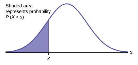
The area to the right is then \(P(X > x) = 1 – P(X < x)\). Remember, \(P(X < x) =\) Area to the left of the vertical line through \(x\). \(P(X > x) = 1 – P(X < x) =\) Area to the right of the vertical line through \(x\). \(P(X < x)\) is the same as \(P(X \leq x)\) and \(P(X > x)\) is the same as \(P(X \geq x)\) for continuous distributions.
Calculations of Probabilities
Probabilities are calculated using technology. There are instructions given as necessary for for using Excel.To calculate the probability, use the probability tables provided in [link] without the use of technology. The tables include instructions for how to use them.
If the area to the left is 0.0228, then the area to the right is \(1 - 0.0228 = 0.9772\).
If the area to the left of \(x\) is \(0.012\), then what is the area to the right?
- Answer
-
\(1 - 0.012 = 0.988\)
The final exam scores in a statistics class were normally distributed with a mean of 63 and a standard deviation of five.
- Find the probability that a randomly selected student scored more than 65 on the exam.
- Find the probability that a randomly selected student scored less than 85.
- Find the 90th percentile (that is, find the score \(k\) that has 90% of the scores below k and 10% of the scores above \(k\)).
- Find the 70th percentile (that is, find the score \(k\) such that 70% of scores are below \(k\) and 30% of the scores are above \(k\)).
Answer
a. Let \(X\) = a score on the final exam. \(X \sim N(63, 5)\), where \(\mu = 63\) and \(\sigma = 5\)
Draw a graph.
Then, find \(P(x > 65)\).
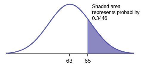
Find the \(z\)-score.
\[z = \frac{65 – 63}{5} = \frac{2}{5} = 0.4\nonumber \]
This tells us that
\[P(x > 65) = P(z > 0.4)\nonumber \]
Before technology, the \(z\)-score was looked up in a standard normal probability table (because the math involved is too cumbersome) to find the probability. Now it's more common to find these values using a statistical software, a spreadsheet software, or a calculator. In this book, examples will be shown using Excel. An appendix is included on information using tables. Both Excel and a standard normal table generally give area to the left of the \(z\)-score.
Find the probability for a student scoring 65.
Excel's formulas automatically calculate the area to the left of a given \(z\)-score. But this example wants an area to the right.
The equation follows the format =NORM.S.DIST(z,cumulative)wherezis the \(z\)-score calculated andcumulativewill always be true.
To find the area to the left: Enter=NORM.S.DIST(0.4,true)which gives 0.6554. So,
\[P(x < 65) = P(z < 0.4) = 0.6554\nonumber \]
However, this problem wants us to find \(P(x > 65)\). Since this is a probability distribution, the total area under the curve is 1. To find the area on the right, we can take the total area, which is 1 and subtract from it the area on the left.
\[P(x > 65) = P(z > 0.4) = 1 – 0.6554 = 0.3446\nonumber \]
Alternatively, we can do all this directly in Excel by entering in =1-NORM.S.DIST(0.4,true)
The probability that a randomly selected student scored more than 65 is 0.3446.
To find the probability that a selected student scored more than 65, subtract the percentile from 1.
Answer
b. Draw a graph.
Then find \(P(x < 85)\), and shade the graph.
Find the \(z\)-score.
\[z = \frac{85 – 63}{5} = \frac{22}{5} = 4.4\nonumber \]
Using Excel, find \(P(x < 85) = P(z < 4.4) = 1\).
\(=\text{NORM.S.DIST}(4.4,\text{true}) = 1\) (rounds to one)
The probability that one student scores less than 85 is approximately one (or 100%).
Answer
c. Find the 90th percentile. For each problem or part of a problem, draw a new graph. Draw the \(x\)-axis. Shade the area that corresponds to the 90th percentile.
Let \(k =\) the 90th percentile. The variable \(k\) is located on the \(x\)-axis. \(P(x < k)\) is the area to the left of \(k\). The 90th percentile \(k\) separates the exam scores into those that are the same or lower than \(k\) and those that are the same or higher. Ninety percent of the test scores are the same or lower than \(k\), and ten percent are the same or higher. The variable \(k\) is often called a critical value.
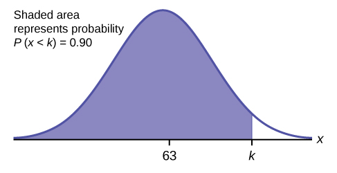
To find this \(z\)-score using Excel, use the formula =NORM.S.INV(probability)
For this problem, \(=\text{NORM.S.INV}(0.90) = 1.28\)
Then use this \(z\)-score to convert back to the corresponding \(x\)-value
\[1.28 = \frac{x – 63}{5}\nonumber \]
\[6.4 = x - 63\nonumber \]
\[69.4 = x\nonumber \]
The 90th percentile is 69.4. This means that 90% of the test scores fall at or below 69.4 and 10% fall at or above.
Answer
d. Find the 70th percentile.
Draw a new graph and label it appropriately. \(=\text{NORM.S.INV}(0.70) = 0.52\)
\[0.52 = \frac{x – 63}{5}\nonumber \]
\[2.6 = x - 63\nonumber \]
\[65.6 = x\nonumber \]
The 70th percentile is 65.6. This means that 70% of the test scores fall at or below 65.6 and 30% fall at or above.
The golf scores for a school team were normally distributed with a mean of 68 and a standard deviation of three. Find the probability that a randomly selected golfer scored less than 65.
- Answer
-
\(Z\)-score: \(z = \frac{65 - 68}{3} = \frac{-3}{3} = -1\)
Excel: \(=\text{NORM.S.DIST}(-1,\text{true}) = 0.1587\)
A personal computer is used for office work at home, research, communication, personal finances, education, entertainment, social networking, and a myriad of other things. Suppose that the average number of hours a household personal computer is used for entertainment is two hours per day. Assume the times for entertainment are normally distributed and the standard deviation for the times is half an hour.
- Find the probability that a household personal computer is used for entertainment between 1.8 and 2.75 hours per day.
- Find the maximum number of hours per day that the bottom quartile of households uses a personal computer for entertainment.
Answer
a. Let \(X =\) the amount of time (in hours) a household personal computer is used for entertainment. \(X \sim N(2, 0.5)\) where \(\mu = 2\) and \(\sigma = 0.5\).
Find \(P(1.8 < x < 2.75)\).
The probability for which you are looking is the area between \(x = 1.8\) and \(x = 2.75\).
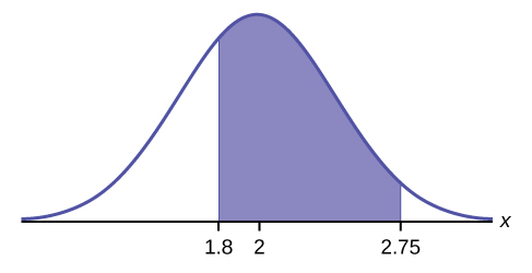
Find the \(z\)-scores for both values
\[z = \frac{2.75 - 2}{0.5} = \frac{0.75}{0.5} = 1.5\nonumber \]
And
\[z = \frac{1.8 - 2}{0.5} = \frac{-0.2}{0.5} = -0.4\nonumber \]
Find the area to the left of the larger \(z\)-score and subtract the area to the left of the smaller \(z\)-score from it.
\[=\text{NORM.S.DIST}(1.5,\text{true}) - \text{NORM.S.DIST}(-0.4,\text{true}) = 0.5886\nonumber \]
The probability that a household personal computer is used between 1.8 and 2.75 hours per day for entertainment is 0.5886.
b.
To find the maximum number of hours per day that the bottom quartile of households uses a personal computer for entertainment, find the 25th percentile, \(k\), where \(P(x < k) = 0.25\).
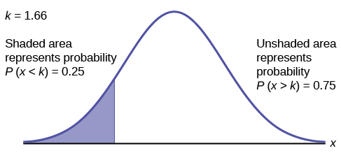
\[=\text{NORM.S.INV}(0.25) = -0.67\nonumber \]
Calculate the \(x\)-value corresponding to the \(z\)-score -0.67
\[-0.674 = \frac{x - 2}{0.5}\nonumber \]
\[-0.34 = x-2\nonumber \]
\[1.66 = x\nonumber \]
The maximum number of hours per day that the bottom quartile of households uses a personal computer for entertainment is 1.66 hours.
The golf scores for a school team were normally distributed with a mean of 68 and a standard deviation of three. Find the probability that a golfer scored between 66 and 70.
- Answer
-
\(Z\)-score: \(z = \frac{70 - 68}{3} = \frac{2}{3} = 0.6667 \)
And \(z = \frac{66 - 68}{3} = \frac{-2}{3} = -0.6667\)
Excel: \(=\text{NORM.S.DIST}(0.6667,\text{true}) - \text{NORM.S.DIST}(-0.6667,\text{true})= 0.4950\)
There are approximately one billion smartphone users in the world today. In the United States the ages 13 to 55+ of smartphone users approximately follow a normal distribution with approximate mean and standard deviation of 36.9 years and 13.9 years, respectively.
- Determine the probability that a random smartphone user in the age range 13 to 55+ is between 23 and 64.7 years old.
- Determine the probability that a randomly selected smartphone user in the age range 13 to 55+ is at most 50.8 years old.
- Find the 80th percentile of this distribution, and interpret it in a complete sentence.
Answer
- \(Z\)-score: \(z = \frac{64.7 - 36.9}{13.9} = \frac{27.8}{13.9} = 2\)
And \(z = \frac{23 - 36.9}{13.9} = \frac{-13.9}{13.9} = -1\)
Excel: \(=\text{NORM.S.DIST}(2,\text{true}) - \text{NORM.S.DIST}(-1,\text{true}) = 0.8186\)
b. \(Z\)-score: \(z = \frac{50.8 - 36.9}{13.9} = \frac{13.9}{13.9} = 1\)
Excel: \(=\text{NORM.S.DIST}(1,\text{true}) = 0.8413\)
c. Excel: \(=\text{NORM.S.INV}(0.80) = 0.84\)
\(Z\)-score: \(0.84 = \frac{x - 36.9}{13.9}\)
\(11.7 = x - 36.9\)
\(48.6 = x\)
The 80th percentile is 48.6 years.
80% of the smartphone users in the age range 13 – 55+ are 48.6 years old or less.
Use the information in Example to answer the following questions.
- Find the 30th percentile, and interpret it in a complete sentence.
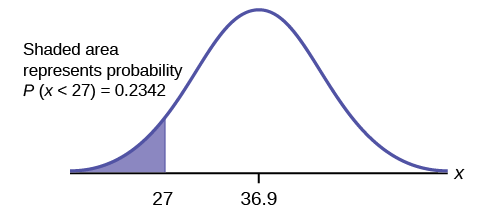
- What is the probability that the age of a randomly selected smartphone user in the range 13 to 55+ is less than 27 years old.
- Answer
-
Let \(X =\) a smart phone user whose age is 13 to 55+. \(X \sim N(36.9, 13.9)\)
To find the 30th percentile, find \(k\) such that \(P(x < k) = 0.30\).Excel: \(=\text{NORM.S.INV}(0.30) = -0.52\)
\(Z\)-score: \(-0.52 = \frac{x - 36.9}{13.9}\)
\(-7.23 = x - 36.9\)
\(29.67 = x\)
The 30th percentile is 29.7 years.
Thirty percent of smartphone users 13 to 55+ are at most 29.7 years and 70% are at least 29.7 years.Find \(P(x < 27)\).
\(Z\)-score: \(z = \frac{27 - 36.9}{13.9} = \frac{-9.9}{13.9} = -0.71\)Excel: \(=\text{NORM.S.DIST}(-0.71,\text{true}) = 0.2389\)
(Note that the two answers differ only by 0.0047.)
In the United States the ages 13 to 55+ of smartphone users approximately follow a normal distribution with approximate mean and standard deviation of 36.9 years and 13.9 years respectively. Using this information, answer the following questions (round answers to one decimal place).
- Calculate the interquartile range (\(IQR\)).
- Forty percent of the ages that range from 13 to 55+ are at least what age?
Answer
a.
\[IQR = Q_{3} – Q_{1}\nonumber \]
Calculate \(Q_{3} =\) 75th percentile and \(Q_{1} =\) 25th percentile.
b.
Find \(k\) where \(P(x > k) = 0.40\) ("At least" translates to "greater than or equal to.")
\(0.40 =\) the area to the right.
Area to the left \(= 1 – 0.40\).
\(=\text{NORM.S.INV}(1-0.40) = 0.25\).
\(Z\)-score: \(0.2533 = \frac{x - 36.9}{13.9}\)
\(3.52 = x - 36.9\)
\(40.42 = x\)
\(k = 40.42\).
Forty percent of the smartphone users from 13 to 55+ are at least 40.4 years.
Two thousand students took an exam. The scores on the exam have an approximate normal distribution with a mean \(\mu = 81\) points and standard deviation \(\sigma = 15\) points.
- Calculate the first- and third-quartile scores for this exam.
- The middle 50% of the exam scores are between what two values?
- Answer
-
a.
\(Q_{1} =\) 25th percentile \(= \text{NORM.S.INV}(0.25) = -0.6745\)
\(Z\)-score: \(-0.6745 = \frac{x - 81}{15}\)
\(-10.12 = x - 81\)
\(70.88 = x\)
\(Q_{3} =\) 75th percentile \(= \text{NORM.S.INV}(0.75) = 0.6745\)
\(Z\)-score: \(0.6745 = \frac{x - 81}{15}\)
\(10.12 = x - 81\)
\(91.12 = x\)
b.
The middle 50% of the scores are between 70.9 and 91.1.
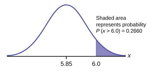
A citrus farmer who grows mandarin oranges finds that the diameters of mandarin oranges harvested on his farm follow a normal distribution with a mean diameter of 5.85 cm and a standard deviation of 0.24 cm.
- Find the probability that a randomly selected mandarin orange from this farm has a diameter larger than 6.0 cm. Sketch the graph.
- The middle 20% of mandarin oranges from this farm have diameters between ______ and ______.
- Find the 90th percentile for the diameters of mandarin oranges, and interpret it in a complete sentence.
Answer
a. \(Z\)-score: \(z = \frac{6 - 5.85}{0.24} = \frac{0.15}{13.9} = 0.625\)
This is asking for the probability to the right, so this is a right tail calculation. Subtract the area given (in Excel) on the left from 1 to find the area on the right.
Excel: \(=1-\text{NORM.S.DIST}(0.625,\text{true}) = 0.2660\)
Answer
b.
\(1 – 0.20 = 0.80\)
The tails of the graph of the normal distribution each have an area of 0.40.
Find \(k1\), the 40th percentile, and \(k2\), the 60th percentile (\(0.40 + 0.20 = 0.60\)).
Excel: \(k1 = \text{NORM.S.INV}(0.40) = -0.25335\) cm
\(Z\)-score: \(-0.25335 = \frac{x - 5.85}{0.24}\)
\(-0.0608 = x - 5.85\)
\(5.79 \text{cm}= x\)
Excel: \(k2 = \text{NORM.S.INV}(0.60) = 0.25335\) cm
\(Z\)-score: \(0.25335 = \frac{x - 5.85}{0.24}\)
\(0.0608 = x - 5.85\)
\(5.91 \text{cm} = x\)
Answer
c. 6.16: Ninety percent of the diameter of the mandarin oranges is at most 6.15 cm.
Using the information from Example, answer the following:
- The middle 45% of mandarin oranges from this farm are between ______ and ______.
- Find the 16th percentile and interpret it in a complete sentence.
- Answer a
-
The middle area \(= 0.45\), so each tail has an area of 0.275.
\( 1 – 0.45 = 0.55\)
The tails of the graph of the normal distribution each have an area of 0.275.
Find \(k1\), the 27.5th percentile and \(k2\), the 72.5th percentile (\(0.45 + 0.275 = 0.725\)).
Excel: \(k1 = \text{NORM.S.INV}(0.275) = -0.59776\) cm
\(Z\)-score: \(-0.59776 = \frac{x - 5.85}{0.24}\)
\(-0.1435 = x - 5.85\)
\(5.71 \text{cm}= x\)
Excel: \(k2 = \text{NORM.S.INV}(0.725) = 0.59776\) cm
\(Z\)-score: \(0.59776 = \frac{x - 5.85}{0.24}\)
\(0.1435 = x - 5.85\)
\(5.99 \text{cm} = x\)
- Answer b
-
Excel: \( = \text{NORM.S.INV}(0.16) = -0.99446\) cm
\(Z\)-score: \(-0.99446 = \frac{x - 5.85}{0.24}\)
\(-0.2387 = x - 5.85\)
\(5.61 \text{cm} = x\)
Sixteen percent of the diameter of the mandarin oranges is at most 5.61 cm.
References
- “Naegele’s rule.” Wikipedia. Available online at http://en.Wikipedia.org/wiki/Naegele's_rule (accessed May 14, 2013).
- “403: NUMMI.” Chicago Public Media & Ira Glass, 2013. Available online at www.thisamericanlife.org/radi...sode/403/nummi (accessed May 14, 2013).
- “Scratch-Off Lottery Ticket Playing Tips.” WinAtTheLottery.com, 2013. Available online at www.winatthelottery.com/publi...partment40.cfm (accessed May 14, 2013).
- “Smart Phone Users, By The Numbers.” Visual.ly, 2013. Available online at http://visual.ly/smart-phone-users-numbers (accessed May 14, 2013).
- “Facebook Statistics.” Statistics Brain. Available online at http://www.statisticbrain.com/facebo...tics/(accessed May 14, 2013).
Review
The normal distribution, which is continuous, is the most important of all the probability distributions. Its graph is bell-shaped. This bell-shaped curve is used in almost all disciplines. Since it is a continuous distribution, the total area under the curve is one. The parameters of the normal are the mean \(\mu\) and the standard deviation σ. A special normal distribution, called the standard normal distribution is the distribution of z-scores. Its mean is zero, and its standard deviation is one.
Formula Review
- Normal Distribution: \(X \sim N(\mu, \sigma)\) where \(\mu\) is the mean and σ is the standard deviation.
- Standard Normal Distribution: \(Z \sim N(0, 1)\).
- Excel function for left tail probability: = NORM.S.DIST(\(z\), true)
- Excel function for the \(k\)th percentile: \(k \)= NORM.S.INV(probability)
Contributors and Attributions
Barbara Illowsky and Susan Dean (De Anza College) with many other contributing authors. Content produced by OpenStax College is licensed under a Creative Commons Attribution License 4.0 license. Download for free at http://cnx.org/contents/30189442-699...b91b9de@18.114.


