5.1: Introduction

Last updated
Save as PDF

Page ID: 20036

\( \newcommand{\vecs}[1]{\overset { \scriptstyle \rightharpoonup} {\mathbf{#1}} } \) \( \newcommand{\vecd}[1]{\overset{-\!-\!\rightharpoonup}{\vphantom{a}\smash {#1}}} \)\(\newcommand{\id}{\mathrm{id}}\) \( \newcommand{\Span}{\mathrm{span}}\) \( \newcommand{\kernel}{\mathrm{null}\,}\) \( \newcommand{\range}{\mathrm{range}\,}\) \( \newcommand{\RealPart}{\mathrm{Re}}\) \( \newcommand{\ImaginaryPart}{\mathrm{Im}}\) \( \newcommand{\Argument}{\mathrm{Arg}}\) \( \newcommand{\norm}[1]{\| #1 \|}\) \( \newcommand{\inner}[2]{\langle #1, #2 \rangle}\) \( \newcommand{\Span}{\mathrm{span}}\) \(\newcommand{\id}{\mathrm{id}}\) \( \newcommand{\Span}{\mathrm{span}}\) \( \newcommand{\kernel}{\mathrm{null}\,}\) \( \newcommand{\range}{\mathrm{range}\,}\) \( \newcommand{\RealPart}{\mathrm{Re}}\) \( \newcommand{\ImaginaryPart}{\mathrm{Im}}\) \( \newcommand{\Argument}{\mathrm{Arg}}\) \( \newcommand{\norm}[1]{\| #1 \|}\) \( \newcommand{\inner}[2]{\langle #1, #2 \rangle}\) \( \newcommand{\Span}{\mathrm{span}}\)\(\newcommand{\AA}{\unicode[.8,0]{x212B}}\)

CHAPTER OBJECTIVES

By the end of this chapter, the student should be able to:

Recognize and understand discrete probability distribution functions, in general.
Calculate and interpret expected values.
Recognize and understand continuous probability density functions in general.
Recognize the normal probability distribution.

A student takes a ten-question, true-false quiz. Because the student had such a busy schedule, he or she could not study and guesses randomly at each answer. What is the probability of the student passing the test with at least a 70%?
Small companies might be interested in the number of long-distance phone calls their employees make during the peak time of the day. Suppose the average is 20 calls. What is the probability that the employees make more than 20 long-distance phone calls during the peak time?

These two examples illustrate two different types of probability problems involving discrete random variables. Recall that discrete data are data that you can count. A random variable describes the outcomes of a statistical experiment in words. The values of a random variable can vary with each repetition of an experiment.

alt — Figure \(\PageIndex{1}\) You can use probability and discrete random variables to calculate the likelihood of lightning striking the ground five times during a half-hour thunderstorm. (Credit: Leszek Leszczynski)

Random Variable Notation

Upper case letters such as \(X\) or \(Y\) denote a random variable. Lower case letters like \(x\) or \(y\) denote the value of a random variable. If \(X\) is a random variable, then \(X\) is written in words, and x is given as a number.

For example, let \(X =\) the number of heads you get when you toss three fair coins. The sample space for the toss of three fair coins is TTT; THH; HTH; HHT; HTT; THT; TTH; HHH. Then, \(x =\) 0, 1, 2, 3. \(X\) is in words and x is a number. Notice that for this example, the \(x\) values are countable outcomes. Because you can count the possible values that \(X\) can take on and the outcomes are random (the x values 0, 1, 2, 3), \(X\) is a discrete random variable.

Probability Distributions

Continuous random variables have many applications. Baseball batting averages, IQ scores, the length of time a long distance telephone call lasts, the amount of money a person carries, the length of time a computer chip lasts, and SAT scores are just a few. The field of reliability depends on a variety of continuous random variables.

The values of discrete and continuous random variables can be ambiguous. For example, if \(X\) is equal to the number of miles (to the nearest mile) you drive to work, then \(X\) is a discrete random variable. You count the miles. If \(X\) is the distance you drive to work, then you measure values of \(X\) and \(X\) is a continuous random variable. For a second example, if \(X\) is equal to the number of books in a backpack, then \(X\) is a discrete random variable. If \(X\) is the weight of a book, then \(X\) is a continuous random variable because weights are measured. How the random variable is defined is very important.

The image shows radish plants of various heights sprouting out of dirt. — Figure \(\PageIndex{2}\): The heights of these radish plants are continuous random variables. (Credit: Rev Stan)

Properties of Continuous Probability Distributions

The graph of a continuous probability distribution is a curve. Probability is represented by area under the curve. The curve is called the probability density function (abbreviated as pdf). We use the symbol \(f(x)\) to represent the curve. \(f(x)\) is the function that corresponds to the graph; we use the density function \(f(x)\) to draw the graph of the probability distribution. Area under the curve is given by a different function called the cumulative distribution function(abbreviated as cdf). The cumulative distribution function is used to evaluate probability as area.

The outcomes are measured, not counted.
The entire area under the curve and above the x-axis is equal to one.
Probability is found for intervals of \(x\) values rather than for individual \(x\) values.
\(P(c < x < d)\) is the probability that the random variable \(X\) is in the interval between the values \(c\) and \(d\). \(P(c < x < d)\) is the area under the curve, above the x-axis, to the right of \(c\) and the left of \(d\).
\(P(x = c) = 0\) The probability that \(x\) takes on any single individual value is zero. The area below the curve, above the x-axis, and between \(x = c\) and \(x = c\) has no width, and therefore no area (area = 0). Since the probability is equal to the area, the probability is also zero.
\(P(c < x < d)\) is the same as \(P(c \leq x \leq d)\) because probability is equal to area.

We will find the area that represents probability by using geometry, formulas, technology, or probability tables. In general, calculus is needed to find the area under the curve for many probability density functions. When we use formulas to find the area in this textbook, the formulas were found by using the techniques of integral calculus. However, because most students taking this course have not studied calculus, we will not be using calculus in this textbook. There are many continuous probability distributions. When using a continuous probability distribution to model probability, the distribution used is selected to model and fit the particular situation in the best way.

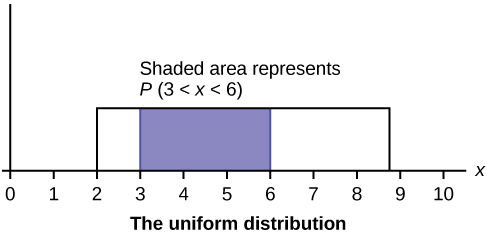
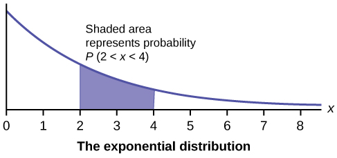
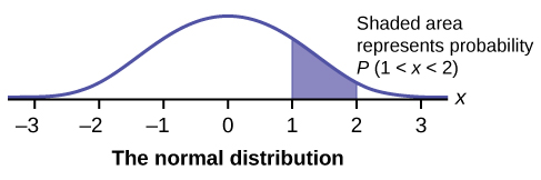
In this chapter and the next, we will study the uniform distribution, the exponential distribution, and the normal distribution. The following graphs illustrate these distributions.

Figure \(\PageIndex{3}\): The graph shows a Uniform Distribution with the area between \(x = 3\) and \(x = 6\) shaded to represent the probability that the value of the random variable \(X\) is in the interval between three and six.

Figure \(\PageIndex{4}\): The graph shows an Exponential Distribution with the area between \(x = 2\) and \(x = 4\) shaded to represent the probability that the value of the random variable \(X\) is in the interval between two and four.

Figure \(\PageIndex{5}\): The graph shows the Standard Normal Distribution with the area between \(x = 1\) and \(x = 2\) shaded to represent the probability that the value of the random variable \(X\) is in the interval between one and two.

Collaborative Exercise

Toss a coin ten times and record the number of heads. After all members of the class have completed the experiment (tossed a coin ten times and counted the number of heads), fill in Table. Let \(X =\) the number of heads in ten tosses of the coin.

\(x\)	Frequency of \(x\)	Relative Frequency of \(x\)

Which value(s) of \(x\) occurred most frequently?
If you tossed the coin 1,000 times, what values could \(x\) take on? Which value(s) of \(x\) do you think would occur most frequently?
What does the relative frequency column sum to?

Glossary

Uniform Distribution: a continuous random variable (RV) that has equally likely outcomes over the domain, \(a < x < b\); it is often referred as the rectangular distribution because the graph of the pdf has the form of a rectangle. Notation: \(X \sim U(a,b)\). The mean is \(\mu = \frac{a+b}{2}\) and the standard deviation is \(\sigma = \sqrt{\frac{(b-a)^{2}}{12}}\). The probability density function is \(f(x) = \frac{1}{b-a}\) for \(a < x < b\) or \(a \leq x \leq b\). The cumulative distribution is \(P(X \leq x) = \frac{x-a}{b-a}\).

Exponential Distribution: a continuous random variable (RV) that appears when we are interested in the intervals of time between some random events, for example, the length of time between emergency arrivals at a hospital; the notation is \(X \sim \text{Exp}(m)\). The mean is \(\mu = \frac{1}{m}\) and the standard deviation is \(\sigma = \frac{1}{m}\). The probability density function is \(f(x) = me^{-mx}\), \(x \geq 0\) and the cumulative distribution function is \(P(X \leq x) = 1 − e^{mx}\).

Contributors and Attributions

Barbara Illowsky and Susan Dean (De Anza College) with many other contributing authors. Content produced by OpenStax College is licensed under a Creative Commons Attribution License 4.0 license. Download for free at http://cnx.org/contents/30189442-699...b91b9de@18.114.