5.4: The Binomial Distribution

Everyone is familiar with a multiple-choice test. Each question has a fixed number of possible answers but only one of them is correct. If we don’t know anything about the question then we can still succeed if we guess the correct answer. What is the chance that we can pass the test just by guessing?

We can answer this by setting up a mathematical model that describes this situation. This is an example of a particular scenario called the Binomial Distribution. We can identify 4 specific characteristics of this problem:

1)    There is an event with only 2 possible outcomes: success and failure. [This is the guess for a particular question.]

2)    The event is repeated a fixed number of times ("trials") with exactly the same chance of success. [This is the number of questions. The chance of success = 1/number of choices]

3)    Each separate repetition is independent of all the others. [Questions are independent of each other]

To make it specific, consider that there are 4 possible answers for each question and that there are 10 questions on the test.

Set \(p\) = probability of success (guessing the correct answer on one question)

       \(n\) = the number of questions

\(p = 0.25\).

\(n = 10\)

The “score”, which is the number of correct answers, we denote by a random variable X.

We can set up a probability distribution table for X by listing all of the possible scores k = 0,1,2,…,9,10 together with their probabilities:

Values for k (Possible scores)	P(X=k)
0
1
2
3
4
5
6
7
8
9
10

 

 

The binomial distribution is frequently used to model the number of successes in a sample of size \(n\) drawn with replacement from a population of size \(N\).

Three characteristics of a binomial experiment

1. There are a fixed number of trials. Think of trials as repetitions of an experiment. The letter \(n\) denotes the number of trials.
2. There are only two possible outcomes, called "success" and "failure," for each trial. The letter \(p\) denotes the probability of a success on one trial, and \(q\) denotes the probability of a failure on one trial. \(p + q = 1\).
3. The \(n\) trials are independent and are repeated using identical conditions. Because the \(n\) trials are independent, the outcome of one trial does not help in predicting the outcome of another trial. Another way of saying this is that for each individual trial, the probability, \(p\), of a success and probability, \(q\), of a failure remain the same. For example, randomly guessing at a true-false statistics question has only two outcomes. If a success is guessing correctly, then a failure is guessing incorrectly. Suppose Joe always guesses correctly on any statistics true-false question with probability \(p = 0.6\). Then, \(q = 0.4\). This means that for every true-false statistics question Joe answers, his probability of success (\(p = 0.6\)) and his probability of failure (\(q = 0.4\)) remain the same.

The outcomes of a binomial experiment fit a binomial probability distribution. The random variable \(X =\) the number of successes obtained in the \(n\) independent trials. The mean, \(\mu\), and variance, \(\sigma^{2}\), for the binomial probability distribution are

\[\mu = np\]

and

\[\sigma^{2} = npq.\]

The standard deviation, \(\sigma\), is then

\[\sigma = \sqrt{npq}.\]

Any experiment that has characteristics two and three and where \(n = 1\) is called a Bernoulli Trial (named after Jacob Bernoulli who, in the late 1600s, studied them extensively). A binomial experiment takes place when the number of successes is counted in one or more Bernoulli Trials.

Example \(\PageIndex{1}\)

At ABC College, the withdrawal rate from an elementary physics course is 30% for any given term. This implies that, for any given term, 70% of the students stay in the class for the entire term. A "success" could be defined as an individual who withdrew. The random variable \(X =\) the number of students who withdraw from the randomly selected elementary physics class.

Example \(\PageIndex{2}\)

Suppose you play a game that you can only either win or lose. The probability that you win any game is 55%, and the probability that you lose is 45%. Each game you play is independent. If you play the game 20 times, write the function that describes the probability that you win 15 of the 20 times. Here, if you define \(X\) as the number of wins, then \(X\) takes on the values 0, 1, 2, 3, ..., 20. The probability of a success is \(p = 0.55\). The probability of a failure is \(q = 0.45\). The number of trials is \(n = 20\). The probability question can be stated mathematically as \(P(x = 15)\).

Example \(\PageIndex{3}\)

A fair coin is flipped 15 times. Each flip is independent. What is the probability of getting more than ten heads? Let \(X =\) the number of heads in 15 flips of the fair coin. \(X\) takes on the values 0, 1, 2, 3, ..., 15. Since the coin is fair, \(p = 0.5\) and \(q = 0.5\). The number of trials is \(n = 15\). State the probability question mathematically.

Solution

\(P(x > 10)\)

Example \(\PageIndex{5}\)

Approximately 70% of statistics students do their homework in time for it to be collected and graded. Each student does homework independently. In a statistics class of 50 students, what is the probability that at least 40 will do their homework on time? Students are selected randomly.

1. This is a binomial problem because there is only a success or a __________, there are a fixed number of trials, and the probability of a success is 0.70 for each trial.
2. If we are interested in the number of students who do their homework on time, then how do we define \(X\)?
3. What values does \(x\) take on?
4. What is a "failure," in words?
5. If \(p + q = 1\), then what is \(q\)?
6. The words "at least" translate as what kind of inequality for the probability question \(P(x\) ____ \(40\)).

Solution

1. failure
2. \(X\) = the number of statistics students who do their homework on time
3. 0, 1, 2, …, 50
4. Failure is defined as a student who does not complete his or her homework on time. The probability of a success is \(p = 0.70\). The number of trials is \(n = 50\).
5. \(q = 0.30\)
6. greater than or equal to (\(\geq\)). The probability question is \(P(x \geq 40)\).

Notation for the Binomial: \(B =\) Binomial Probability Distribution Function

\[X \sim B(n, p)\]

Read this as "\(X\) is a random variable with a binomial distribution." The parameters are \(n\) and \(p\); \(n =\) number of trials, \(p =\) probability of a success on each trial.

Example \(\PageIndex{6}\)

It has been stated that about 41% of adult workers have a high school diploma but do not pursue any further education. If 20 adult workers are randomly selected, find the probability that at most 12 of them have a high school diploma but do not pursue any further education. How many adult workers do you expect to have a high school diploma but do not pursue any further education?

Let \(X\) = the number of workers who have a high school diploma but do not pursue any further education.

\(X\) takes on the values 0, 1, 2, ..., 20 where \(n = 20, p = 0.41\), and \(q = 1 – 0.41 = 0.59\). \(X \sim B(20, 0.41)\)

Find \(P(x \leq 12)\). \(P(x \leq 12) = 0.9738\). (calculator or computer)

Go into 2^nd DISTR. The syntax for the instructions are as follows:

To calculate (\(x = \text{value}): \text{binompdf}(n, p, \text{number}\)) if "number" is left out, the result is the binomial probability table.

To calculate \(P(x \leq \text{value}): \text{binomcdf}(n, p, \text{number})\) if "number" is left out, the result is the cumulative binomial probability table.

For this problem: After you are in 2^nd DISTR, arrow down to binomcdf. Press ENTER. Enter 20,0.41,12). The result is \(P(x \leq 12) = 0.9738\).

If you want to find \(P(x = 12)\), use the pdf (binompdf). If you want to find \(P(x > 12)\), use \(1 - \text{binomcdf}(20,0.41,12)\).

The probability that at most 12 workers have a high school diploma but do not pursue any further education is 0.9738.

The graph of \(X \sim B(20, 0.41)\) is as follows:

Figure \(\PageIndex{1}\) : The graph of \(X \sim B(20, 0.41)\).

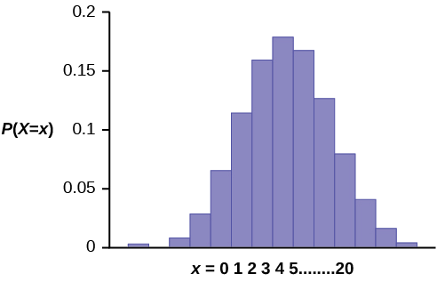
The y-axis contains the probability of \(x\), where \(X =\) the number of workers who have only a high school diploma.

The number of adult workers that you expect to have a high school diploma but not pursue any further education is the mean, \(\mu = np = (20)(0.41) = 8.2\).

The formula for the variance is \(\sigma^{2} = npq\). The standard deviation is \(\sigma = \sqrt{npq}\).

\[\sigma = \sqrt{(20)(0.41)(0.59)} = 2.20.\].9695\)

Example \(\PageIndex{7}\)

In the 2013 Jerry’s Artarama art supplies catalog, there are 560 pages. Eight of the pages feature signature artists. Suppose we randomly sample 100 pages. Let \(X =\) the number of pages that feature signature artists.

1. What values does \(x\) take on?
2. What is the probability distribution? Find the following probabilities:
   1. the probability that two pages feature signature artists
   2. the probability that at most six pages feature signature artists
   3. the probability that more than three pages feature signature artists.
3. Using the formulas, calculate the (i) mean and (ii) standard deviation.

Answer

1. \(x = 0, 1, 2, 3, 4, 5, 6, 7, 8\)
2. \(X \sim B(100,8560)(100,8560)\)
   1. \(P(x = 2) = \text{binompdf}\left(100,\dfrac{8}{560},2\right) = 0.2466\)
   2. \(P(x \leq 6) = \text{binomcdf}\left(100,\dfrac{8}{560},6\right) = 0.9994\)
   3. \(P(x > 3) = 1 – P(x \leq 3) = 1 – \text{binomcdf}\left(100,\dfrac{8}{560},3\right) = 1 – 0.9443 = 0.0557\)
3. 1. Mean \(= np = (100)\left(\dfrac{8}{560}\right) = \dfrac{800}{560} \approx 1.4286\)
   2. Standard Deviation \(= \sqrt{npq} = \sqrt{(100)\left(\dfrac{8}{560}\right)\left(\dfrac{552}{560}\right)} \approx 1.1867\)

Example \(\PageIndex{8}\)

The lifetime risk of developing pancreatic cancer is about one in 78 (1.28%). Suppose we randomly sample 200 people. Let \(X\) = the number of people who will develop pancreatic cancer.

1. What is the probability distribution for \(X\)?
2. Using the formulas, calculate the (i) mean and (ii) standard deviation of \(X\).
3. Use your calculator to find the probability that at most eight people develop pancreatic cancer
4. Is it more likely that five or six people will develop pancreatic cancer? Justify your answer numerically.

Answer

1. \(X \sim B(200, 0.0128)\)
2. 1. Mean \(= np = 200(0.0128) = 2.56\)
   2. Standard Deviation \(= \sqrt{npq} = \sqrt{(200)(0.0128)(0.9872)} \approx 1.5897\)
3. Using the TI-83, 83+, 84 calculator with instructions as provided in Example:
   \(P(x \leq 8) = \text{binomcdf}(200, 0.0128, 8) = 0.9988\)
4. \(P(x = 5) = \text{binompdf}(200, 0.0128, 5) = 0.0707\)
   \(P(x = 6) = \text{binompdf}(200, 0.0128, 6) = 0.0298\)
   So \(P(x = 5) > P(x = 6)\); it is more likely that five people will develop cancer than six.

Example \(\PageIndex{9}\)

The following example illustrates a problem that is not binomial. It violates the condition of independence. ABC College has a student advisory committee made up of ten staff members and six students. The committee wishes to choose a chairperson and a recorder. What is the probability that the chairperson and recorder are both students? The names of all committee members are put into a box, and two names are drawn without replacement. The first name drawn determines the chairperson and the second name the recorder. There are two trials. However, the trials are not independent because the outcome of the first trial affects the outcome of the second trial. The probability of a student on the first draw is \(\dfrac{6}{16}\). The probability of a student on the second draw is \(\dfrac{5}{15}\), when the first draw selects a student. The probability is \(\dfrac{6}{15}\), when the first draw selects a staff member. The probability of drawing a student's name changes for each of the trials and, therefore, violates the condition of independence.

WeBWorK Problems

Query \(\PageIndex{1}\)

}\)

Query \(\PageIndex{2}\)

Query \(\PageIndex{3}\)

Query \(\PageIndex{4}\)

Query \(\PageIndex{5}\)

Query \(\PageIndex{6}\)

 

References

1. “Access to electricity (% of population),” The World Bank, 2013. Available online at http://data.worldbank.org/indicator/...first&sort=asc (accessed May 15, 2015).
2. “Distance Education.” Wikipedia. Available online at http://en.Wikipedia.org/wiki/Distance_education (accessed May 15, 2013).
3. “NBA Statistics – 2013,” ESPN NBA, 2013. Available online at http://espn.go.com/nba/statistics/_/seasontype/2 (accessed May 15, 2013).
4. Newport, Frank. “Americans Still Enjoy Saving Rather than Spending: Few demographic differences seen in these views other than by income,” GALLUP® Economy, 2013. Available online at http://www.gallup.com/poll/162368/am...-spending.aspx (accessed May 15, 2013).
5. Pryor, John H., Linda DeAngelo, Laura Palucki Blake, Sylvia Hurtado, Serge Tran. The American Freshman: National Norms Fall 2011. Los Angeles: Cooperative Institutional Research Program at the Higher Education Research Institute at UCLA, 2011. Also available online at http://heri.ucla.edu/PDFs/pubs/TFS/N...eshman2011.pdf (accessed May 15, 2013).
6. “The World FactBook,” Central Intelligence Agency. Available online at www.cia.gov/library/publicat...k/geos/af.html (accessed May 15, 2013).
7. “What are the key statistics about pancreatic cancer?” American Cancer Society, 2013. Available online at www.cancer.org/cancer/pancrea...key-statistics (accessed May 15, 2013).

Review

A statistical experiment can be classified as a binomial experiment if the following conditions are met:

There are a fixed number of trials, \(n\).

There are only two possible outcomes, called "success" and, "failure" for each trial. The letter \(p\) denotes the probability of a success on one trial and \(q\) denotes the probability of a failure on one trial.

The \(n\) trials are independent and are repeated using identical conditions.

The outcomes of a binomial experiment fit a binomial probability distribution. The random variable \(X =\) the number of successes obtained in the \(n\) independent trials. The mean of \(X\) can be calculated using the formula \(\mu = np\), and the standard deviation is given by the formula \(\sigma = \sqrt{npq}\).

Formula Review

• \(X \sim B(n, p)\) means that the discrete random variable \(X\) has a binomial probability distribution with \(n\) trials and probability of success \(p\).
• \(X =\) the number of successes in \(n\) independent trials
• \(n =\) the number of independent trials
• \(X\) takes on the values \(x = 0, 1, 2, 3, \dotsc, n\)
• \(p =\) the probability of a success for any trial
• \(q =\) the probability of a failure for any trial
• \(p + q = 1\)
• \(q = 1 – p\)

The mean of \(X\) is \(\mu = np\). The standard deviation of \(X\) is \(\sigma = \sqrt{npq}\).

Contributors and Attributions

• Barbara Illowsky and Susan Dean (De Anza College) with many other contributing authors. Content produced by OpenStax College is licensed under a Creative Commons Attribution License 4.0 license. Download for free at http://cnx.org/contents/30189442-699...b91b9de@18.114.

Use the following information to answer the next eight exercises: The Higher Education Research Institute at UCLA collected data from 203,967 incoming first-time, full-time freshmen from 270 four-year colleges and universities in the U.S. 71.3% of those students replied that, yes, they believe that same-sex couples should have the right to legal marital status. Suppose that you randomly pick eight first-time, full-time freshmen from the survey. You are interested in the number that believes that same sex-couples should have the right to legal marital status.

 

Glossary

Binomial Experiment

a statistical experiment that satisfies the following three conditions:

1. There are a fixed number of trials, \(n\).
2. There are only two possible outcomes, called "success" and, "failure," for each trial. The letter \(p\) denotes the probability of a success on one trial, and \(q\) denotes the probability of a failure on one trial.
3. The \(n\) trials are independent and are repeated using identical conditions.

Bernoulli Trials

an experiment with the following characteristics:

1. There are only two possible outcomes called “success” and “failure” for each trial.
2. The probability \(p\) of a success is the same for any trial (so the probability \(q = 1 − p\) of a failure is the same for any trial).

Binomial Probability Distribution

a discrete random variable (RV) that arises from Bernoulli trials; there are a fixed number, \(n\), of independent trials. “Independent” means that the result of any trial (for example, trial one) does not affect the results of the following trials, and all trials are conducted under the same conditions. Under these circumstances the binomial RV \(X\) is defined as the number of successes in \(n\) trials. The notation is: \(X ~ B(n, p)\). The mean is \(\mu = np\) and the standard deviation is \(\sigma = \sqrt{npq}\). The probability of exactly \(x\) successes in \(n\) trials is
\(P(X = x) = {n \choose x}p^{x}q^{n-x}\).