2.7: Measures of Spread- Variance and Standard Deviation

[NOTE from VS: The following is pulled from Shafer and Zhang]

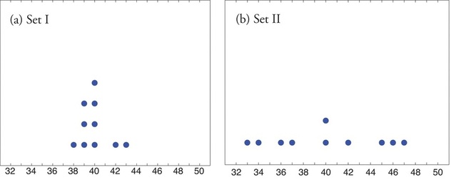
Look at the two data sets in Table 2.7.1 and the graphical representation of each, called a dot plot, in Figure 2.7.1.

Table 2.7.1: Two Data Sets

Data Set I:	40	38	42	40	39	39	43	40	39	40
Data Set II:	46	37	40	33	42	36	40	47	34	45

The two sets of ten measurements each center at the same value: they both have mean, median, and mode equal to 40. Nevertheless a glance at the figure shows that they are markedly different. In Data Set I the measurements vary only slightly from the center, while for Data Set II the measurements vary greatly. Just as we have attached numbers to a data set to locate its center, we now wish to associate to each data set numbers that measure quantitatively how the data either scatter away from the center or cluster close to it. These new quantities are called measures of variability, and we will discuss three of them.

Figure 2.7.1: Dot Plots of Data Sets

The Range

First we discuss the simplest measure of variability.

Definition: range

The range \(R\) of a data set is difference between its largest and smallest values \[R=x_{\text{max}}−x_{\text{min}}\] where \(\displaystyle x_{\text{max}}\) is the largest measurement in the data set and \(\displaystyle x_{\text{min}}\) is the smallest.

Example \(\PageIndex{1}\): Identifyig the Range of a dataset

Find the range of each data set in Table \(\PageIndex{1}\).

Solution:

• For Data Set I the maximum is \(43\) and the minimum is \(38\), so the range is \(R=43−38=5\).
• For Data Set II the maximum is \(47\) and the minimum is \(33\), so the range is \(R=47−33=14\).

The range is a measure of variability because it indicates the size of the interval over which the data points are distributed. A smaller range indicates less variability (less dispersion) among the data, whereas a larger range indicates the opposite. The range is very limited in the information it gives us, as it is only based on the largest and smallest values. Anything can happen in between and the range tells us nothing about these. In order to get information about how all of the data points are spread out we can compare each one to the mean. We do this with the "Variance" and "Standard Deviation".

The Variance and the Standard Deviation

The other two measures of variability that we will consider are the Variance and the Standard Deviation. They are intimately connected, as the standard deviation is just the square root of the variance. The word "deviation" gives us the clue of what we are trying to do. In order to measure how much variation there is in the data, we use the mean as the central value and then calculate all of the differences ("deviations") of each data value from the mean. The Variance is easier to calculate because it does not involve the square root. It has a drawback in that the quantities used are squared, so it will not represent the correct units for the data. The Standard Deviation takes the square root of the Variance and so the squared units are returned to regular units (such as inches, pounds and so forth based on the sampled data0.

Calculating the Standard Deviation

If \(x\) is a number, then the difference "\(x\) – mean" is called its deviation. In a data set, there are as many deviations as there are items in the data set. The deviations are used to calculate the standard deviation. If the numbers belong to a population, in symbols a deviation is \(x - \mu\). For sample data, in symbols a deviation is \(x - \bar{x}\).

To calculate the standard deviation, we need to calculate the variance first, and then take the square root. The variance is the average of the squares of the deviations (the \(x - \bar{x}\) values for a sample, or the \(x - \mu\) values for a population). The symbol \(\sigma^{2}\) represents the population variance; the population standard deviation \(\sigma\) is the square root of the population variance. The symbol \(s^{2}\) represents the sample variance; the sample standard deviation s is the square root of the sample variance. You can think of the standard deviation as a special average of the deviations.

If the numbers come from a census of the entire population and not a sample, when we calculate the average of the squared deviations to find the variance, we divide by \(N\), the number of items in the population. If the data are from a sample rather than a population, when we calculate the average of the squared deviations, we divide by n – 1, one less than the number of items in the sample.

In summary, the procedure to calculate the standard deviation depends on whether the numbers are the entire population or are data from a sample. The calculations are the same except that for the sample we divide by "sample size - 1: n-1" and for the population we divide by "Population size N". Therefore the symbol used to represent the standard deviation depends on whether it is calculated from a population or a sample. The lower case letter s represents the sample standard deviation and the Greek letter \(\sigma\) (sigma, lower case) represents the population standard deviation. If the sample has the same characteristics as the population, then s should be a good estimate of \(\sigma\).

Formulas for the Sample Standard Deviation

\[s = \sqrt{\dfrac{\sum(x-\bar{x})^{2}}{n-1}} \label{eq1}\]

For the sample standard deviation, the denominator is \(n - 1\), that is the sample size MINUS 1.

Formulas for the Population Standard Deviation

\[\sigma = \sqrt{\dfrac{\sum(x-\mu)^{2}}{N}} \label{eq3} \]

For the population standard deviation, the denominator is \(N\), the number of items in the population.

The Sample Variance is the calculation before taking the square root.

Definition: sample variance and sample Standard Deviation

The sample variance of a set of \(n\) sample data is the number \(\mathbf{ s^2}\) defined by the formula

\[s^2 = \dfrac{\sum (x-\bar x)^2}{n-1}\]

An algebraically equivalent formula is sometimes used, because the calculations are easier to perform:

\[s^2=\dfrac{\sum x^2 - \dfrac{1}{n}\left(\sum x\right)^2}{n-1}\]

The square root \(\mathbf s\) of the sample variance is called the sample standard deviation of a set of \(n\) sample data . It is given by the formulas

\[s = \sqrt{s^2} = \sqrt{\dfrac{\sum (x-\bar x)^2}{n-1} } = \sqrt{\dfrac{\sum x^2 - \dfrac{1}{n}\left(\sum x\right)^2}{n-1}}.\]

Although the first formula in each case looks less complicated than the second, the latter is easier to use in hand computations, and is called a shortcut formula.

Example \(\PageIndex{2}\): Identifying the Variance and Standard Deviation of a Dataset

Find the sample variance and the sample standard deviation of Data Set II in Table \(\PageIndex{1}\).

Solution

To use the defining formula (the first formula) in the definition we first compute for each observation \(x\) its deviation \(x-\bar x\) from the sample mean. Since the mean of the data is \(\bar x =40\), we obtain the ten numbers displayed in the second line of the supplied table

\[ \begin{array}{c|cccccccccc} x & 46 & 37 & 40 & 33 & 42 & 36 & 40 & 47 & 34 & 45 \\ \hline x−\bar{x} & -6 & -3 & 0 & -7 & 2 & -4 & 0 & 7 & -6 & 5 \end{array} \nonumber\]

Thus

\[\sum (x-\bar{x})^2=6^2+(-3)^2+0^2+(-7)^2+2^2+(-4)^2+0^2+7^2+(-6)^2+5^2=224\nonumber\]

so the variance is

\[s^2=\dfrac{\sum (x-\bar{x})^2}{n-1}=\dfrac{224}{9}=24.\bar{8} \nonumber\]

and the standard deviation is

\[s=\sqrt{24.\bar{8}} \approx 4.99 \nonumber\]

The student is encouraged to compute the ten deviations for Data Set I and verify that their squares add up to \(20\), so that the sample variance and standard deviation of Data Set I are the much smaller numbers

\[s^2=20/9=2.\bar{2}\]

and

\[s=20/9 \approx 1.49\]

The standard deviation

• provides a numerical measure of the overall amount of variation in a data set, and
• can be used to determine whether a particular data value is close to or far from the mean.

WeBWorK Problems

2.7.1

2.7.2

2.7.3

2.7.4

2.7.5

The number of standard deviations a data value is from the mean can be used as a measure of the closeness of a data value to the mean. Because the standard deviation measures the spread of the data this gives a uniform measure for any data set.

For example: suppose that Rosa and Binh both shop at supermarket A. Rosa waits at the checkout counter for seven minutes and Binh waits for one minute. At supermarket A, the mean waiting time is five minutes and the standard deviation is two minutes.

Rosa waits for seven minutes:

• This is two minutes longer than the average wait time. 
• Two minutes is the same as one standard deviation.
• Rosa's wait time of seven minutes is one standard deviation above the average of five minutes.

Binh waits for one minute.

• This is four minutes less than the average of five; four minutes is equal to two standard deviations.
• Binh's wait time of one minute is two standard deviations below the average of five minutes.
• A "rule of thumb" is that more than two standard deviations away from the average is considered "far from the average". In general, the shape of the distribution of the data affects how much of the data is further away than two standard deviations. (You will learn more about this in later chapters.)

The number line may help you understand standard deviation. If we were to put five and seven on a number line, seven is to the right of five. We say, then, that seven is one standard deviation to the right of five because \(5 + (1)(2) = 7\).

If one were also part of the data set, then one is two standard deviations to the left of five because \(5 + (-2)(2) = 1\).

Figure \(\PageIndex{1}\)

• In general, a value = mean + (#ofSTDEV)(standard deviation)
• where #ofSTDEVs = the number of standard deviations
• #ofSTDEV does not need to be an integer
• One is two standard deviations less than the mean of five because: \(1 = 5 + (-2)(2)\).

The equation value = mean + (#ofSTDEVs)(standard deviation) can be expressed for a sample and for a population.

• sample: \[x = \bar{x} + \text{(#ofSTDEV)(s)}\]
• Population: \[x = \mu + \text{(#ofSTDEV)(s)}\]

The lower case letter s represents the sample standard deviation and the Greek letter \(\sigma\) (sigma, lower case) represents the population standard deviation.

The symbol \(\bar{x}\) is the sample mean and the Greek symbol \(\mu\) is the population mean.

In practice, USE A CALCULATOR OR COMPUTER SOFTWARE TO CALCULATE THE STANDARD DEVIATION. If you are using a TI-83, 83+, 84+ calculator, you need to select the appropriate standard deviation \(\sigma_{x}\) or \(s_{x}\) from the summary statistics. We will concentrate on using and interpreting the information that the standard deviation gives us. However you should study the following step-by-step example to help you understand how the standard deviation measures variation from the mean. (The calculator instructions appear at the end of this example.)

Example \(\PageIndex{1}\)

In a fifth grade class, the teacher was interested in the average age and the sample standard deviation of the ages of her students. The following data are the ages for a SAMPLE of n = 20 fifth grade students. The ages are rounded to the nearest half year:

9; 9.5; 9.5; 10; 10; 10; 10; 10.5; 10.5; 10.5; 10.5; 11; 11; 11; 11; 11; 11; 11.5; 11.5; 11.5;

\[\bar{x} = \dfrac{9+9.5(2)+10(4)+10.5(4)+11(6)+11.5(3)}{20} = 10.525 \nonumber\]

The average age is 10.53 years, rounded to two places.

The variance may be calculated by using a table. Then the standard deviation is calculated by taking the square root of the variance. We will explain the parts of the table after calculating s.

Data	Freq.	Deviations	Deviations^2	(Freq.)(Deviations^2)
x	f	(x – \(\bar{x}\))	(x – \(\bar{x}\))2	(f)(x – \(\bar{x}\))2
9	1	9 – 10.525 = –1.525	(–1.525)2 = 2.325625	1 × 2.325625 = 2.325625
9.5	2	9.5 – 10.525 = –1.025	(–1.025)^2 = 1.050625	2 × 1.050625 = 2.101250
10	4	10 – 10.525 = –0.525	(–0.525)^2 = 0.275625	4 × 0.275625 = 1.1025
10.5	4	10.5 – 10.525 = –0.025	(–0.025)^2 = 0.000625	4 × 0.000625 = 0.0025
11	6	11 – 10.525 = 0.475	(0.475)^2 = 0.225625	6 × 0.225625 = 1.35375
11.5	3	11.5 – 10.525 = 0.975	(0.975)^2 = 0.950625	3 × 0.950625 = 2.851875
				The total is 9.7375

The sample variance, \(s^{2}\), is equal to the sum of the last column (9.7375) divided by the total number of data values minus one (20 – 1):

\[s^{2} = \dfrac{9.7375}{20-1} = 0.5125 \nonumber\]

The sample standard deviation s is equal to the square root of the sample variance:

\[s = \sqrt{0.5125} = 0.715891 \nonumber\]

and this is rounded to two decimal places, \(s = 0.72\).

Typically, you do the calculation for the standard deviation on your calculator or computer. The intermediate results are not rounded. This is done for accuracy.

• For the following problems, recall that value = mean + (#ofSTDEVs)(standard deviation). Verify the mean and standard deviation or a calculator or computer.
• For a sample: \(x\) = \(\bar{x}\) + (#ofSTDEVs)(s)
• For a population: \(x\) = \(\mu\) + (#ofSTDEVs)\(\sigma\)
• For this example, use x = \(\bar{x}\) + (#ofSTDEVs)(s) because the data is from a sample

1. Verify the mean and standard deviation on your calculator or computer.
2. Find the value that is one standard deviation above the mean. Find (\(\bar{x}\) + 1s).
3. Find the value that is two standard deviations below the mean. Find (\(\bar{x}\) – 2s).
4. Find the values that are 1.5 standard deviations from (below and above) the mean.

Solution

1. • Clear lists L1 and L2. Press STAT 4:ClrList. Enter 2nd 1 for L1, the comma (,), and 2nd 2 for L2.
   • Enter data into the list editor. Press STAT 1:EDIT. If necessary, clear the lists by arrowing up into the name. Press CLEAR and arrow down.
   • Put the data values (9, 9.5, 10, 10.5, 11, 11.5) into list L1 and the frequencies (1, 2, 4, 4, 6, 3) into list L2. Use the arrow keys to move around.
   • Press STAT and arrow to CALC. Press 1:1-VarStats and enter L1 (2nd 1), L2 (2nd 2). Do not forget the comma. Press ENTER.
   • \(\bar{x}\) = 10.525
   • Use Sx because this is sample data (not a population): Sx=0.715891
2. (\(\bar{x} + 1s) = 10.53 + (1)(0.72) = 11.25\)
3. \((\bar{x} - 2s) = 10.53 – (2)(0.72) = 9.09\)
4. • \((\bar{x} - 1.5s) = 10.53 – (1.5)(0.72) = 9.45\)
   • \((\bar{x} + 1.5s) = 10.53 + (1.5)(0.72) = 11.61\)

Explanation of the standard deviation calculation shown in the table

The deviations show how spread out the data are about the mean. The data value 11.5 is farther from the mean than is the data value 11 which is indicated by the deviations 0.97 and 0.47. A positive deviation occurs when the data value is greater than the mean, whereas a negative deviation occurs when the data value is less than the mean. The deviation is –1.525 for the data value nine. If you add the deviations, the sum is always zero. (For Example \(\PageIndex{1}\), there are \(n = 20\) deviations.) So you cannot simply add the deviations to get the spread of the data. By squaring the deviations, you make them positive numbers, and the sum will also be positive. The variance, then, is the average squared deviation.

The variance is a squared measure and does not have the same units as the data. Taking the square root solves the problem. The standard deviation measures the spread in the same units as the data.

Notice that instead of dividing by \(n = 20\), the calculation divided by \(n - 1 = 20 - 1 = 19\) because the data is a sample. For the sample variance, we divide by the sample size minus one (\(n - 1\)). Why not divide by \(n\)? The answer has to do with the population variance. The sample variance is an estimate of the population variance. Based on the theoretical mathematics that lies behind these calculations, dividing by (\(n - 1\)) gives a better estimate of the population variance.

Your concentration should be on what the standard deviation tells us about the data. The standard deviation is a number which measures how far the data are spread from the mean. Let a calculator or computer do the arithmetic.

The standard deviation, \(s\) or \(\sigma\), is either zero or larger than zero. When the standard deviation is zero, there is no spread; that is, all the data values are equal to each other. The standard deviation is small when the data are all concentrated close to the mean, and is larger when the data values show more variation from the mean. When the standard deviation is a lot larger than zero, the data values are very spread out about the mean; outliers can make \(s\) or \(\sigma\) very large.

The standard deviation, when first presented, can seem unclear. By graphing your data, you can get a better "feel" for the deviations and the standard deviation. You will find that in symmetrical distributions, the standard deviation can be very helpful but in skewed distributions, the standard deviation may not be much help. The reason is that the two sides of a skewed distribution have different spreads. In a skewed distribution, it is better to look at the first quartile, the median, the third quartile, the smallest value, and the largest value. Because numbers can be confusing, always graph your data. Display your data in a histogram or a box plot.

Example \(\PageIndex{2}\)

Use the following data (first exam scores) from Susan Dean's spring pre-calculus class:

33; 42; 49; 49; 53; 55; 55; 61; 63; 67; 68; 68; 69; 69; 72; 73; 74; 78; 80; 83; 88; 88; 88; 90; 92; 94; 94; 94; 94; 96; 100

1. Create a chart containing the data, frequencies, relative frequencies, and cumulative relative frequencies to three decimal places.
2. Calculate the following to one decimal place using a TI-83+ or TI-84 calculator:
   1. The sample mean
   2. The sample standard deviation
   3. The median
   4. The first quartile
   5. The third quartile
   6. IQR
3. Construct a box plot and a histogram on the same set of axes. Make comments about the box plot, the histogram, and the chart.

Answer

1. See Table
2. 1. The sample mean = 73.5
   2. The sample standard deviation = 17.9
   3. The median = 73
   4. The first quartile = 61
   5. The third quartile = 90
   6. IQR = 90 – 61 = 29
3. The \(x\)-axis goes from 32.5 to 100.5; \(y\)-axis goes from -2.4 to 15 for the histogram. The number of intervals is five, so the width of an interval is (\(100.5 - 32.5\)) divided by five, is equal to 13.6. Endpoints of the intervals are as follows: the starting point is 32.5, \(32.5 + 13.6 = 46.1\), \(46.1 + 13.6 = 59.7\), \(59.7 + 13.6 = 73.3\), \(73.3 + 13.6 = 86.9\), \(86.9 + 13.6 = 100.5 =\) the ending value; No data values fall on an interval boundary.

Figure \(\PageIndex{2}\).

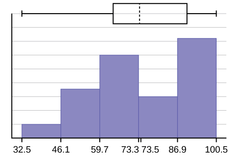
The long left whisker in the box plot is reflected in the left side of the histogram. The spread of the exam scores in the lower 50% is greater (\(73 - 33 = 40\)) than the spread in the upper 50% (\(100 - 73 = 27\)). The histogram, box plot, and chart all reflect this. There are a substantial number of A and B grades (80s, 90s, and 100). The histogram clearly shows this. The box plot shows us that the middle 50% of the exam scores (IQR = 29) are Ds, Cs, and Bs. The box plot also shows us that the lower 25% of the exam scores are Ds and Fs.

Data	Frequency	Relative Frequency	Cumulative Relative Frequency
33	1	0.032	0.032
42	1	0.032	0.064
49	2	0.065	0.129
53	1	0.032	0.161
55	2	0.065	0.226
61	1	0.032	0.258
63	1	0.032	0.29
67	1	0.032	0.322
68	2	0.065	0.387
69	2	0.065	0.452
72	1	0.032	0.484
73	1	0.032	0.516
74	1	0.032	0.548
78	1	0.032	0.580
80	1	0.032	0.612
83	1	0.032	0.644
88	3	0.097	0.741
90	1	0.032	0.773
92	1	0.032	0.805
94	4	0.129	0.934
96	1	0.032	0.966
100	1	0.032	0.998 (Why isn't this value 1?)

Standard deviation of Grouped Frequency Tables

Recall that for grouped data we do not know individual data values, so we cannot describe the typical value of the data with precision. In other words, we cannot find the exact mean, median, or mode. We can, however, determine the best estimate of the measures of center by finding the mean of the grouped data with the formula:

\[\text{Mean of Frequency Table} = \dfrac{\sum fm}{\sum f}\]

where \(f\) interval frequencies and \(m =\) interval midpoints.

Just as we could not find the exact mean, neither can we find the exact standard deviation. Remember that standard deviation describes numerically the expected deviation a data value has from the mean. In simple English, the standard deviation allows us to compare how “unusual” individual data is compared to the mean.

Example \(\PageIndex{3}\)

Find the standard deviation for the data in Table \(\PageIndex{3}\).

Table \(\PageIndex{3}\)

Class	Frequency, f	Midpoint, m	m^2	\(\bar{x}\)	fm^2	Standard Deviation
0–2	1	1	1	7.58	1	3.5
3–5	6	4	16	7.58	96	3.5
6–8	10	7	49	7.58	490	3.5
9–11	7	10	100	7.58	700	3.5
12–14	0	13	169	7.58	0	3.5
15–17	2	16	256	7.58	512	3.5

For this data set, we have the mean, \(\bar{x}\) = 7.58 and the standard deviation, \(s_{x}\) = 3.5. This means that a randomly selected data value would be expected to be 3.5 units from the mean. If we look at the first class, we see that the class midpoint is equal to one. This is almost two full standard deviations from the mean since 7.58 – 3.5 – 3.5 = 0.58. While the formula for calculating the standard deviation is not complicated, \(s_{x} = \sqrt{\dfrac{f(m - \bar{x})^{2}}{n-1}}\) where \(s_{x}\) = sample standard deviation, \(\bar{x}\) = sample mean, the calculations are tedious. It is usually best to use technology when performing the calculations.

Comparing Values from Different Data Sets

The standard deviation is useful when comparing data values that come from different data sets. If the data sets have different means and standard deviations, then comparing the data values directly can be misleading.

• For each data value, calculate how many standard deviations away from its mean the value is.
• Use the formula: value = mean + (#ofSTDEVs)(standard deviation); solve for #ofSTDEVs.
• \(\text{#ofSTDEVs} = \dfrac{\text{value-mean}}{\text{standard deviation}}\)
• Compare the results of this calculation.

#ofSTDEVs is often called a "z-score"; we can use the symbol \(z\). In symbols, the formulas become:

Sample	\(x = \bar{x} + zs\)
Population	\(x = \mu + z\sigma\)

Example \(\PageIndex{4}\)

Two students, John and Ali, from different high schools, wanted to find out who had the highest GPA when compared to his school. Which student had the highest GPA when compared to his school?

Student	GPA	School Mean GPA	School Standard Deviation
John	2.85	3.0	0.7
Ali	77	80	10

Answer

For each student, determine how many standard deviations (#ofSTDEVs) his GPA is away from the average, for his school. Pay careful attention to signs when comparing and interpreting the answer.

\[z = \text{#ofSTDEVs} = \left(\dfrac{\text{value-mean}}{\text{standard deviation}}\right) = \left(\dfrac{x + \mu}{\sigma}\right) \nonumber\]

For John,

\[z = \text{#ofSTDEVs} = \left(\dfrac{2.85-3.0}{0.7}\right) = -0.21 \nonumber\]

For Ali,

\[z = \text{#ofSTDEVs} = (\dfrac{77-80}{10}) = -0.3 \nonumber\]

John has the better GPA when compared to his school because his GPA is 0.21 standard deviations below his school's mean while Ali's GPA is 0.3 standard deviations below his school's mean.

John's z-score of –0.21 is higher than Ali's z-score of –0.3. For GPA, higher values are better, so we conclude that John has the better GPA when compared to his school.

The following lists give a few facts that provide a little more insight into what the standard deviation tells us about the distribution of the data.

For ANY data set, no matter what the distribution of the data is:

• At least 75% of the data is within two standard deviations of the mean.
• At least 89% of the data is within three standard deviations of the mean.
• At least 95% of the data is within 4.5 standard deviations of the mean.
• This is known as Chebyshev's Rule.

For data having a distribution that is BELL-SHAPED and SYMMETRIC:

• Approximately 68% of the data is within one standard deviation of the mean.
• Approximately 95% of the data is within two standard deviations of the mean.
• More than 99% of the data is within three standard deviations of the mean.
• This is known as the Empirical Rule.
• It is important to note that this rule only applies when the shape of the distribution of the data is bell-shaped and symmetric. We will learn more about this when studying the "Normal" or "Gaussian" probability distribution in later chapters.

References

1. Data from Microsoft Bookshelf.
2. King, Bill.“Graphically Speaking.” Institutional Research, Lake Tahoe Community College. Available online at www.ltcc.edu/web/about/institutional-research (accessed April 3, 2013).

Review

The standard deviation can help you calculate the spread of data. There are different equations to use if are calculating the standard deviation of a sample or of a population.

• The Standard Deviation allows us to compare individual data or classes to the data set mean numerically.
• \(s = \sqrt{\dfrac{\sum(x-\bar{x})^{2}}{n-1}}\) or \(s = \sqrt{\dfrac{\sum f (x-\bar{x})^{2}}{n-1}}\) is the formula for calculating the standard deviation of a sample. To calculate the standard deviation of a population, we would use the population mean, \(\mu\), and the formula \(\sigma = \sqrt{\dfrac{\sum(x-\mu)^{2}}{N}}\) or \(\sigma = \sqrt{\dfrac{\sum f (x-\mu)^{2}}{N}}\).∑​f(x−μ)2N−−−−−−−−−√.

Formula Review

\[s_{x} = \sqrt{\dfrac{\sum fm^{2}}{n} - \bar{x}^2}\]

where \(s_{x} \text{sample standard deviation}\) and \(\bar{x} = \text{sample mean}\)

Use the following information to answer the next two exercises: The following data are the distances between 20 retail stores and a large distribution center. The distances are in miles.

29; 37; 38; 40; 58; 67; 68; 69; 76; 86; 87; 95; 96; 96; 99; 106; 112; 127; 145; 150

Glossary

Standard Deviation

a number that is equal to the square root of the variance and measures how far data values are from their mean; notation: s for sample standard deviation and σ for population standard deviation.

Variance

mean of the squared deviations from the mean, or the square of the standard deviation; for a set of data, a deviation can be represented as \(x\) – \(\bar{x}\) where \(x\) is a value of the data and \(\bar{x}\) is the sample mean. The sample variance is equal to the sum of the squares of the deviations divided by the difference of the sample size and one.

Contributors and Attributions

Barbara Illowsky and Susan Dean (De Anza College) with many other contributing authors. Content produced by OpenStax College is licensed under a Creative Commons Attribution License 4.0 license. Download for free at http://cnx.org/contents/30189442-699...b91b9de@18.114.