
16.23: Continuous-Time Branching Chains
- Page ID
- 10396

\( \newcommand{\vecs}[1]{\overset { \scriptstyle \rightharpoonup} {\mathbf{#1}} } \)
\( \newcommand{\vecd}[1]{\overset{-\!-\!\rightharpoonup}{\vphantom{a}\smash {#1}}} \)
\( \newcommand{\id}{\mathrm{id}}\) \( \newcommand{\Span}{\mathrm{span}}\)
( \newcommand{\kernel}{\mathrm{null}\,}\) \( \newcommand{\range}{\mathrm{range}\,}\)
\( \newcommand{\RealPart}{\mathrm{Re}}\) \( \newcommand{\ImaginaryPart}{\mathrm{Im}}\)
\( \newcommand{\Argument}{\mathrm{Arg}}\) \( \newcommand{\norm}[1]{\| #1 \|}\)
\( \newcommand{\inner}[2]{\langle #1, #2 \rangle}\)
\( \newcommand{\Span}{\mathrm{span}}\)
\( \newcommand{\id}{\mathrm{id}}\)
\( \newcommand{\Span}{\mathrm{span}}\)
\( \newcommand{\kernel}{\mathrm{null}\,}\)
\( \newcommand{\range}{\mathrm{range}\,}\)
\( \newcommand{\RealPart}{\mathrm{Re}}\)
\( \newcommand{\ImaginaryPart}{\mathrm{Im}}\)
\( \newcommand{\Argument}{\mathrm{Arg}}\)
\( \newcommand{\norm}[1]{\| #1 \|}\)
\( \newcommand{\inner}[2]{\langle #1, #2 \rangle}\)
\( \newcommand{\Span}{\mathrm{span}}\) \( \newcommand{\AA}{\unicode[.8,0]{x212B}}\)
\( \newcommand{\vectorA}[1]{\vec{#1}} % arrow\)
\( \newcommand{\vectorAt}[1]{\vec{\text{#1}}} % arrow\)
\( \newcommand{\vectorB}[1]{\overset { \scriptstyle \rightharpoonup} {\mathbf{#1}} } \)
\( \newcommand{\vectorC}[1]{\textbf{#1}} \)
\( \newcommand{\vectorD}[1]{\overrightarrow{#1}} \)
\( \newcommand{\vectorDt}[1]{\overrightarrow{\text{#1}}} \)
\( \newcommand{\vectE}[1]{\overset{-\!-\!\rightharpoonup}{\vphantom{a}\smash{\mathbf {#1}}}} \)
\( \newcommand{\vecs}[1]{\overset { \scriptstyle \rightharpoonup} {\mathbf{#1}} } \)
\( \newcommand{\vecd}[1]{\overset{-\!-\!\rightharpoonup}{\vphantom{a}\smash {#1}}} \)
\(\newcommand{\avec}{\mathbf a}\) \(\newcommand{\bvec}{\mathbf b}\) \(\newcommand{\cvec}{\mathbf c}\) \(\newcommand{\dvec}{\mathbf d}\) \(\newcommand{\dtil}{\widetilde{\mathbf d}}\) \(\newcommand{\evec}{\mathbf e}\) \(\newcommand{\fvec}{\mathbf f}\) \(\newcommand{\nvec}{\mathbf n}\) \(\newcommand{\pvec}{\mathbf p}\) \(\newcommand{\qvec}{\mathbf q}\) \(\newcommand{\svec}{\mathbf s}\) \(\newcommand{\tvec}{\mathbf t}\) \(\newcommand{\uvec}{\mathbf u}\) \(\newcommand{\vvec}{\mathbf v}\) \(\newcommand{\wvec}{\mathbf w}\) \(\newcommand{\xvec}{\mathbf x}\) \(\newcommand{\yvec}{\mathbf y}\) \(\newcommand{\zvec}{\mathbf z}\) \(\newcommand{\rvec}{\mathbf r}\) \(\newcommand{\mvec}{\mathbf m}\) \(\newcommand{\zerovec}{\mathbf 0}\) \(\newcommand{\onevec}{\mathbf 1}\) \(\newcommand{\real}{\mathbb R}\) \(\newcommand{\twovec}[2]{\left[\begin{array}{r}#1 \\ #2 \end{array}\right]}\) \(\newcommand{\ctwovec}[2]{\left[\begin{array}{c}#1 \\ #2 \end{array}\right]}\) \(\newcommand{\threevec}[3]{\left[\begin{array}{r}#1 \\ #2 \\ #3 \end{array}\right]}\) \(\newcommand{\cthreevec}[3]{\left[\begin{array}{c}#1 \\ #2 \\ #3 \end{array}\right]}\) \(\newcommand{\fourvec}[4]{\left[\begin{array}{r}#1 \\ #2 \\ #3 \\ #4 \end{array}\right]}\) \(\newcommand{\cfourvec}[4]{\left[\begin{array}{c}#1 \\ #2 \\ #3 \\ #4 \end{array}\right]}\) \(\newcommand{\fivevec}[5]{\left[\begin{array}{r}#1 \\ #2 \\ #3 \\ #4 \\ #5 \\ \end{array}\right]}\) \(\newcommand{\cfivevec}[5]{\left[\begin{array}{c}#1 \\ #2 \\ #3 \\ #4 \\ #5 \\ \end{array}\right]}\) \(\newcommand{\mattwo}[4]{\left[\begin{array}{rr}#1 \amp #2 \\ #3 \amp #4 \\ \end{array}\right]}\) \(\newcommand{\laspan}[1]{\text{Span}\{#1\}}\) \(\newcommand{\bcal}{\cal B}\) \(\newcommand{\ccal}{\cal C}\) \(\newcommand{\scal}{\cal S}\) \(\newcommand{\wcal}{\cal W}\) \(\newcommand{\ecal}{\cal E}\) \(\newcommand{\coords}[2]{\left\{#1\right\}_{#2}}\) \(\newcommand{\gray}[1]{\color{gray}{#1}}\) \(\newcommand{\lgray}[1]{\color{lightgray}{#1}}\) \(\newcommand{\rank}{\operatorname{rank}}\) \(\newcommand{\row}{\text{Row}}\) \(\newcommand{\col}{\text{Col}}\) \(\renewcommand{\row}{\text{Row}}\) \(\newcommand{\nul}{\text{Nul}}\) \(\newcommand{\var}{\text{Var}}\) \(\newcommand{\corr}{\text{corr}}\) \(\newcommand{\len}[1]{\left|#1\right|}\) \(\newcommand{\bbar}{\overline{\bvec}}\) \(\newcommand{\bhat}{\widehat{\bvec}}\) \(\newcommand{\bperp}{\bvec^\perp}\) \(\newcommand{\xhat}{\widehat{\xvec}}\) \(\newcommand{\vhat}{\widehat{\vvec}}\) \(\newcommand{\uhat}{\widehat{\uvec}}\) \(\newcommand{\what}{\widehat{\wvec}}\) \(\newcommand{\Sighat}{\widehat{\Sigma}}\) \(\newcommand{\lt}{<}\) \(\newcommand{\gt}{>}\) \(\newcommand{\amp}{&}\) \(\definecolor{fillinmathshade}{gray}{0.9}\)Basic Theory
Introduction
Generically, suppose that we have a system of particles that can generate or split into other particles of the same type. Here are some typical examples:
- The particles are biological organisms that reproduce.
- The particles are neutrons in a chain reaction.
- The particles are electrons in an electron multiplier.
We assume that the lifetime of each particle is exponentially distributed with parameter \( \alpha \in (0, \infty) \), and at the end of its life, is replaced by a random number of new particles that we will refer to as children of the original particle. The number of children \( N \) of a particle has probability density function \( f \) on \( \N \). The particles act independently, so in addition to being identically distributed, the lifetimes and the number of children are independent from particle to particle. Finally, we assume that \( f(1) = 0 \), so that a particle cannot simply die and be replaced by a single new particle. Let \( \mu \) and \( \sigma^2 \) denote the mean and variance of the number of offspring of a single particle. So \[ \mu = \E(N) = \sum_{n=0}^\infty n f(n), \quad \sigma^2 = \var(N) = \sum_{n=0}^\infty (n - \mu)^2 f(n) \] We assume that \( \mu \) is finite and so \( \sigma^2 \) makes sense. In our study of discrete-time Markov chains, we studied branching chains in terms of generational time. Here we want to study the model in real time.
Let \( X_t \) denote the number of particles at time \( t \in [0, \infty) \). Then \( \bs{X} = \{X_t: t \in [0, \infty)\} \) is a continuous-time Markov chain on \( \N \), known as a branching chain. The exponential parameter function \( \lambda \) and jump transition matrix \( Q \) are given by
- \( \lambda(x) = \alpha x \) for \( x \in \N \)
- \(Q(x, x + k - 1) = f(k)\) for \( x \in \N_+ \) and \( k \in \N \).
Proof
That \( \bs X \) is a continuous-time Markov chain follows from the assumptions and the basic structure of continuous-time Markov chains. In turns out that the assumption that \( \mu \lt \infty \) implies that \( \bs X \) is regular, so that \( \tau_n \to \infty \) as \( n \to \infty \), where \( \tau_n \) is the time of the \( n \)th jump for \( n \in \N_+ \).
- Starting with \( x \) particles, the time of the first state change is the minimum of \( x \) independent variables, each exponentially distributed with parameter \( \alpha \). As we know, this minimum is also exponentially distributed with parameter \( \alpha x \).
- Starting in state \( x \in \N_+ \), the next state will be \( x + k - 1 \) for \( k \in \N \), if the particle dies and leaves \( k \) children in her place. This happens with probability \( f(k) \).
Of course 0 is an absorbing state, since this state means extinction with no particles. (Note that \( \lambda(0) = 0 \) and so by default, \( Q(0, 0) = 1 \).) So with a branching chain, there are essentially two types of behavior: population extinction or population explosion.
For the branching chain \( \bs X = \{X_t: t \in [0, \infty)\} \) one of the following events occurs with probability 1:
- Extinction: \( X_t = 0 \) for some \( t \in [0, \infty) \) and hence \( X_s = 0 \) for all \( s \ge t \).
- Explosion: \( X_t \to \infty \) as \( t \to \infty \).
Proof
If \( f(0) \gt 0 \) then all states lead to the absorbing state 0 and hence the set of positive staties \( \N_+ \) is transient. With probability 1, the jump chain \( \bs Y \) visits a transient state only finitely many times, so with probability 1 either \( Y_n = 0 \) for some \( n \in \N \) or \( Y_n \to \infty \) as \( n \to \infty \). If \( f(0) = 0 \) then \( Y_n \) is strictly increasing in \( n \), since \( f(1) = 0 \) by assumption. Hence with probability 1, \( Y_n \to \infty \) as \( n \to \infty \).
Without the assumption that \( \mu \lt \infty \), explosion can actually occur in finite time. On the other hand, the assumption that \( f(1) = 0 \) is for convenience. Without this assumption, \( \bs X \) would still be a continuous-time Markov chain, but as discussed in the Introduction, the exponential parameter function would be \( \lambda(x) = \alpha f(1) x \) for \( x \in \N \) and the jump transition matrix would be \[ Q(x, x + k - 1) = \frac{f(k)}{1 - f(1)}, \quad x \in \N_+, \; k \in \{0, 2, 3, \ldots\} \]
Because all particles act identically and independently, the branching chain starting with \( x \in \N_+ \) particles is essentially \( x \) independent copies of the branching chain starting with 1 particle. In many ways, this is the fundamental insight into branching chains, and in particular, means that we can often condition on \( X(0) = 1 \).
Generator and Transition Matrices
As usual, we will let \( \bs P = \{P_t: t \in [0, \infty)\} \) denote the semigroup of transition matrices of \( \bs X \), so that \( P_t(x, y) = \P(X_t = y \mid X = x) \) for \( (x, y) \in \N^2 \). Similarly, \( G \) denotes the infinitesimal generator matrix of \( \bs X \).
The infinitesimal generator \( G \) is given by \begin{align*} G(x, x) & = -\alpha x, \quad x \in \N \\ G(x, x + k - 1) & = \alpha x f( k), \quad x \in \N_+, \, k \in \N \end{align*}
Proof
This follows immediately from the exponential parameter function and the jump transition matrix above.
The Kolmogorov backward equation is \[ \frac{d}{dt} P_t(x, y) = -\alpha x P_t(x, x) + \alpha x \sum_{k=0}^\infty f(k) P_t(x + k - 1, y), \quad (x, y) \in \N^2 \]
Proof
The backward equation is \( \frac{d}{dt} P_t = G P_t \), so the result follows from the previous theorem.
Unlike some of our other continuous-time models, the jump chain \( \bs Y \) governed by \( Q \) is not the discrete-time version of the model. That is, \( \bs Y \) is not a discrete-time branching chain, since in discrete time, the index \( n \) represents the \( n \)th generation, whereas here it represent the \( n \)th time that a particle reproduces. However, there are lots of discrete-time branching chain embedded in the continuous-time chain.
Fix \( t \in (0, \infty) \) and define \( \bs Z_t = \{X_{n t}: n \in \N\} \). Then \( \bs Z_t \) is a discrete-time branching chain with offspring probability density function \( f_t \) given by \( f_t(x) = P_t(1, x) \) for \( x \in \N \).
Proof
In general, we know that sampling a (homogeneous) continuous-time Markov chain at multiples of a fixed \( t \in (0, \infty) \), results in a (homogeneous) discrete-time Markov chain. For \( \bs Z_t \) to be a branching chain, we just need to note that \[ P_t(x, y) = f_t^{*x}(y), \quad (x, y) \in \N^2 \] where \( f_t^{*x} \) is the convolution power of \( f_t \) of order \( x \). This is a consequence of the fundamental fact that \( X_t \) given \( X_0 = x \) has the same distribution as the sum of \( x \) independent copies of \( X_t \) given \( X_0 = 1 \). Recall that the PDF of a sum of independent variables is the convolution of the individual PDFs.
Probability Generating Functions
As in the discrete case, probability generating functions are an important analytic tool for continuous-time branching chains.
For \( t \in [0, \infty) \) let \( \Phi_t \) denote the probability generating function of \( X_t \) given \( X_0 = 1 \) \[ \Phi_t(r) = \E\left(r^{X_t} \mid X_0 = 1\right) = \sum_{x=0}^\infty r^x P_t(1, x) \] Let \( \Psi \) denote the probability generating function of \( N \) \[\Psi(r) = \E\left(r^N\right) = \sum_{n=0}^\infty r^n f(n)\]The generating functions are defined (the series are absolutely convergent) at least for \( r \in (-1, 1] \).
The collection of generating functions \( \bs \Phi = \{\Phi_t: t \in [0, \infty)\} \) gives the same information as the collection of probability density functions \( \{P_t(1, \cdot): t \in [0, \infty)\} \). With the fundamental insight that the branching process starting with one particle determines the branching process in general, \( \bs \Phi \) actually determines the transition semigroup \( \bs P = \{P_t: t \in [0, \infty)\} \).
For \( t \in [0, \infty) \) and \( x \in \N \), the probability generating function of \( X_t \) given \( X_0 = x \) is \( \Phi_t^x \): \[ \sum_{y=0}^\infty r^y P_t(x, y) = [\Phi_t(r)]^x \]
Proof
Again, given \( X_0 = x \), the number of particles \( X_t \) at time \( t \) has the same distribution as the sum of \( x \) independent copies of \( X_t \) given \( X_0 = 1 \). Recall that the PGF of a sum of independent variables is the product of the PGFs of the variables.
Note that \( \Phi_t \) is the generating function of the offspring distribution for the embedded discrete-time branching chain \( \bs Z_t = \{X_{n t}: n \in \N\} \) for \( t \in (0, \infty) \). On the other hand, \( \Psi \) is the generating function of the offspring distribution for the continuous-time chain. So our main goal in this discussion is to see how \( \bs{\Phi} \) is built from \( \Psi \). Because \( \bs P \) is a semigroup under matrix multiplication, and because the particles act identically and independently, \( \bs \Phi \) is a semigroup under composition.
\( \Phi_{s+t} = \Phi_s \circ \Phi_t \) for \( s, \, t \in [0, \infty) \).
Proof
Using the semigroup property (the Chapman-Kolmogorov equations) and the previous result we have \begin{align*} \Phi_{s+t}(r) & = \sum_{y=0}^\infty r^y P_{s+t}(1, y) = \sum_{y=0}^\infty r^y \sum_{x=0}^\infty P_s(1, x) P_t(x, y) = \sum_{x=0}^\infty P_s(1, x) \sum_{y=0}^\infty r^y P_t(x, y) \\ & = \sum_{x=0}^\infty P_s(1, x) [\Phi_t(r)]^x = \Phi_s[\Phi_t(r)] \end{align*}
Note also that \( \Phi_0(r) = \E(r^{X_0} \mid X_0 = 1) = r \) for all \( r \in \R \). This also follows from the semigroup property: \( \Phi_0 = \Phi_0 \circ \Phi_0 \). The fundamental relationship between the collection of generating functions \( \bs \Phi \) and the generating function \( \Psi \) is given in the following theorem:
The mapping \( t \mapsto \Phi_t \) satisfies the differential equation \[ \frac{d}{dt} \Phi_t = \alpha (\Psi \circ \Phi_t - \Phi_t) \]
Proof
Using the Kolmogorov backward equation we have \[ \frac{d}{dt} \Phi_t(r) = \sum_{x=0}^\infty r^x \frac{d}{dt} P_t(1, x) = \sum_{x=0}^\infty r^x G P_t(1, x) \] Using the generator above, \[ G P_t(1, x) = \sum_{y = 0}^\infty G(1, y) P_t(y, x) = - \alpha P_t(1, x) + \sum_{k=0}^\infty \alpha f(k) P_t(k, x), \quad x \in \N \] Substituting and using the result above gives \begin{align*} \frac{d}{dt} \Phi_t(r) & = \sum_{x=0}^\infty r^x \left[-\alpha P_t(1, x) + \sum_{k=0}^\infty \alpha f(k) P_t(k, x)\right] = - \alpha \sum_{x=0}^\infty r^x P_t(1, x) + \alpha \sum_{x=0}^\infty \sum_{k=0}^\infty r^x f(k) P_t(k, x) \\ & = -\alpha \Phi_t(r) + \alpha \sum_{k=0}^\infty f(k) \sum_{x=0}^\infty r^x P_t(k, x) = -\alpha \Psi_t(r) + \alpha \sum_{k=0}^\infty f(k) [\Phi_t(r)]^k = -\alpha \Phi_t(r) + \alpha \Psi[\Phi_t(r)] \end{align*}
This differential equation, along with the initial condition \( \Phi_0(r) = r \) for all \( r \in \R \) determines the collection of generating functions \( \bs \Phi \). In fact, an implicit solution for \( \Phi_t(r) \) is given by the integral equation \[ \int_r^{\Phi_t(r)} \frac{1}{\Psi(u) - u} du = \alpha t \] Another relationship is given in the following theorem. Here, \( \Phi_t^\prime \) refers to the derivative of the generating function \( \Phi_t \) with respect to its argument, of course (so \( r \), not \( t \)).
For \( t \in [0, \infty) \), \[ \Phi_t^\prime = \frac{\Psi \circ \Phi_t - \Phi_t}{\Psi - \Phi_0} \]
Proof
From the semigroup property, we have \( \Phi_{t+s}(r) = \Phi_t[\Phi_s(r)] \) for \( s, \, t \in [0, \infty) \). Differentiating with respect to \( s \) and using the chain rule along with the previous theorem gives \[ \frac{d}{ds} \Phi_{t+s}(r) = \Phi_t^\prime[\Phi_s(r)] \frac{d}{ds} \Phi_s(r) = \Phi_t^\prime[\Phi_s(r)] \alpha \left[ \Psi(\Phi_s(r)) - \Phi_s(r)\right] \] Evaluating at \( s = 0 \) and using the condition \( \Phi_0(r) = r \) we have \[ \frac{d}{dt}\Phi_t(r) = \Phi_t^\prime(r) \alpha [\Psi(r) - r] \] Using the previous theorem once again gives \[ \alpha \left[\Psi(\Phi_t(r)) - \Phi_t(r)\right] = \Phi_t^\prime(r) \alpha[\Psi(r) - r] \] Solving for \( \Phi_t^\prime(r) \) gives the result.
Moments
In this discussion, we wil study the mean and variance of the number of particles at time \( t \in [0, \infty) \). Let \[ m_t = \E(X_t \mid X_0 = 1), \; v_t = \var(X_t \mid X_0 = 1), \quad t \in [0, \infty) \] so that \( m_t \) and \( v_t \) are the mean and variance, starting with a single particle. As always with a branching process, it suffices to consider a single particle:
For \( t \in [0, \infty) \) and \( x \in \N \),
- \( \E(X_t \mid X_0 = x) = x \, m_t \)
- \( \var(X_t \mid X_0 = x) = x \, v_t \)
Proof
Once again, the distribution of \( X_t \) given \( X_0 = x \) is the same as the distribution of the sum of \( x \) independent copies of \( X_t \) given \( X_0 = 1 \). Recall that the mean of a sum of variables is the sum of the individual means, and the variance of the sum of independent variables is the sum of the individual variances.
Recall also that \( \mu \) and \( \sigma^2 \) are the the mean and variance of the number of offspring of a particle. Here is the connection between the means:
\( m_t = e^{\alpha(\mu - 1) t} \) for \( t \in [0, \infty) \).
- If \( \mu \lt 1 \) then \( m_t \to 0 \) as \( t \to \infty \). This is extinction in the mean.
- If \( \mu \gt 1 \) then \( m_t \to \infty \) as \( t \to \infty \). This is explosion in the mean.
- If \( \mu = 1 \) then \( m_t = 1 \) for all \( t \in [0, \infty) \). This is stability in the mean.
Proof
From the proof of the previous theorem, \[ \frac{d}{dt} \Phi_t(r) = \alpha \Phi_t^\prime(r) [\Psi(r) - r] \] Differentiating with respect to \( r \), interchanging the order of integration on the left, and using the product rule on the right gives \[ \frac{d}{dt} \Phi_t^\prime(r) = \alpha \Phi_t^{\prime \prime}(r)[\Psi(r) - r] + \alpha \Phi_t^\prime(r)[\Psi^\prime(r) - 1] \] Now let \( r = 1 \) and recall that \( \Phi(1) = 1 \). We get \[ \frac{d}{dt} \Phi_t^\prime(1) = \alpha \Phi_t^\prime(1)[\Psi^\prime(1) - 1] \] From the basic theory of probability generating functions, \( m_t = \Phi_t^\prime(1) \) and similarly, \( \mu = \Psi^\prime(1) \). Hence we have \[ \frac{d}{dt} m_t = \alpha (\mu - 1) m_t \] Of course we have the initial condition \( m_0 = 1 \).
This result is intuitively very appealing. As a function of time, the expected number of particles either grows or decays exponentially, depending on whether the expected number of offspring of a particle is greater or less than one. The connection between the variances is more complicated. We assume that \( \sigma^2 \lt \infty \).
If \( \mu \ne 1 \) then \[ v_t = \left[\frac{\sigma^2}{\mu - 1} + (\mu - 1)\right]\left[e^{2 \alpha (\mu - 1) t} - e^{\alpha (\mu - 1) t}\right], \quad t \in [0, \infty) \] If \( \mu = 1 \) then \( v_t = \alpha \sigma^2 t \).
- If \( \mu \lt 1 \) then \( v_t \to 0 \) as \( t \to \infty \)
- If \( \mu \ge 1 \) then \( v_t \to \infty \) as \( t \to \infty \)
Proof
Probability generating functions are naturally connected to factorial moments, so it's best to work with these. Thus, let \( w_t = \E[X_t(X_t - 1) \mid X_0 = 1]\) for \( t \in [0, \infty) \) and let \( \delta = \E[N(N - 1)] \). These are the factorial moments of order 2. In the proof of the last theorem we showed that \[ \frac{d}{dt} \Phi_t^\prime(r) = \alpha \Phi_t^{\prime \prime}(r)[\Psi(r) - r] + \alpha \Phi_t^\prime(r)[\Psi^\prime(r) - 1] \] Differentiating with respect to \( r \) again gives \[ \frac{d}{dt} \Phi_t^{\prime \prime}(r) = \alpha \Phi_t^{\prime \prime \prime}(r)[\Psi(r) - r] + 2 \alpha \Phi_t^{\prime \prime}(r)[\Psi^\prime(r) - 1] + \alpha \Phi_t^\prime(r) \Psi^{\prime \prime}(r) \] Now substitute \( r = 1 \). Recall that \( \Phi_t^{\prime \prime}(1) = w_t \), \( \Phi_t^\prime(1) = m_t = e^{\alpha (\mu - 1) t} \), \( \Psi^{\prime \prime}(1) = \delta \), \( \Psi^\prime(1) = \mu \), and \( \Psi(1) = 1 \). We get the differential equation \[ \frac{d}{dt} w_t = 2 \alpha (\mu - 1) w_t + \alpha \delta e^{\alpha (\mu - 1) t} \] with the initial condition \( w_0 = 0 \).
Suppose that \( \mu \ne 1 \). Then using standard methods for a linear, first order differential equations with constant coefficients and an exponential forcing function, the solution is \[ w_t = \frac{\delta}{\mu - 1}\left[e^{2 \alpha (\mu - 1)} - e^{\alpha (\mu - 1) t}\right] \] But \( \delta = \sigma^2 + \mu^2 - \mu \), and similarly \( w_t = v_t + m_t^2 - m_t \) with \( m_t = e^{\alpha (\mu - 1) t} \). Substitution and some algebra then gives the result.
Suppose now that \( \mu = 1 \). Then also \( m_t = 1 \) for all \( t \in [0, \infty) \) and so \( \delta = \sigma^2 \) and \( v_t = w_t \). The differential equation above reduces simply to \[ \frac{d}{dt} v_t = \alpha \sigma^2 \] with initial condition \( v_0 = 0 \) so trivially \( v_t = \alpha \sigma^2 t \). Finally, in the context of part (b), note that if \( \mu = 1 \) we must have \( \sigma^2 \gt 0 \) since we have assumed that \( f(1) = 0 \).
If \( \mu \lt 1 \) so that \( m_t \to 0 \) as \( t \to \infty \) and we have extinction in the mean, then \( v_t \to 0 \) as \( t \to \infty \) also. If \( \mu \gt 1 \) so that \( m_t \to \infty \) as \( t \to \infty \) and we have explosion in the mean, then \( v_t \to \infty \) as \( t \to \infty \) also. We would expect these results. On the other hand, if \( \mu = 1 \) so that \( m_t = 1 \) for all \( t \in [0, \infty) \) and we have stability in the mean, then \( v_t \) grows linearly in \( t \). This gives some insight into what to expect next when we consider the probability of extinction.
The Probability of Extinction
As shown above, there are two types of behavior for a branching process, either population extinction or population explosion. In this discussion, we study the extinction probability, starting as usual with a single particle: \[ q = \P(X_t = 0 \text{ for some } t \in (0, \infty) \mid X_0 = 1) = \lim_{t \to \infty} \P(X_t = 0 \mid X_0 = 1) \] Need we say it? The extinction probability starting with an arbitrary number of particles is easy.
For \( x \in \N \), \[ \P(X_t = 0 \text{ for some } t \in (0, \infty) \mid X_0 = x) = \lim_{t \to \infty} \P(X_t = 0 \mid X_0 = x) = q^x \]
Proof
Given \( X_0 = x \), extinction has occurred by time \( t \) if and only if extinction has occurred by time \( t \) for each of the \( x \) independent branching chains formed from the descendents of the \( x \) initial particles.
We can easily relate extinction for the continuous-time branching chain \( \bs X \) to extinction for any of the embedded discrete-time branching chains.
If extinction occurs for \( \bs X \) then extinction occurs for \( \bs Z_t \) for every \( t \in (0, \infty) \). Conversely if extinction occurs for \( \bs Z_t \) for some \( t \in (0, \infty) \) then extinction occurs for \( \bs Z_t \) for every \( t \in (0, \infty) \) and extinction occurs for \( \bs X \). Hence \( q \) is the minimum solution in \( (0, 1] \) of the equation \(\Phi_t(r) = r\) for every \( t \in (0, \infty) \).
Proof
The statements about the extinction event follow immediately from the fact that \( 0 \) is absorbing, so that if \( X_t = 0 \) for some \( t \in (0, \infty) \) then \( X_s = 0 \) for every \( s \in [t, \infty) \). The result for the extinction probability \( q \) follows from the theory of discrete-time branching chains.
So whether or not extinction is certain depends on the critical parameter \( \mu \).
The extinction probability \( q \) and the mean of the offspring distribution \( \mu \) are related as follows:
- If \( \mu \le 1 \) then \( q = 1 \), so extinction is certain.
- If \( \mu \gt 1 \) then \( 0 \lt q \lt 1 \), so there is a positive probability of extinction and a positive probability of explosion.
Proof
These results follow from the corresponding results for discrete-time branching chains. Fix \( t \in (0, \infty) \) and recall that \( m_t \) is the mean of the offspring distribution for the discrete-time chain \( \bs Z_t = \{X_{nt}: n \in \N\} \). From the result above,
- If \( \mu \le 1 \) then \( m_t \le 1 \).
- If \( \mu \gt 1 \) then \( m_t \gt 1 \).
It would be nice to have an equation for \( q \) in terms of the offspring probability generating function \( \Psi \). This is also easy
The probability of extinction \( q \) is the minimum solution in \( (0, 1] \) of the equation \( \Psi(r) = r \).
Proof
From the result above, \( \Phi_t(q) = 1 \) for every \( t \in (0, \infty) \). Substituting \( r = q \) in the differential equation above, we have \( \frac{d}{dt} \Phi_t(q) = 0 \) and hence \( \Psi(q) = q \). As in the theory of discrete branching chains, the equation \( \Psi(r) = r \) has only the solution 1 in (0, 1] if \( \mu = \Psi^\prime(1) \le 1 \) or there are two solutions \( q \in (0, 1) \) and \( 1 \) if \( \mu \gt 0 \). In both cases, \( q \) is the smaller solution.
Special Models
We now turn our attention to a number of special branching chains that are important in applications or lead to interesting insights. We will use the notation established above, so that \( \alpha \) is the parameter of the exponential lifetime of a particle, \( Q \) is the transition matrix of the jump chain, \( G \) is the infinitesimal generator matrix, and \( P_t \) is the transition matrix at time \( t \in [0, \infty) \). Similarly, \( m_t = \E(X_t \mid X_0 = x) \), \( v_t = \var(X_t \mid X_0 = x) \), and \( \Phi_t \) are the mean, variance, and generating function of the number of particles at time \( t \in [0, \infty) \), starting with a single particle. As always, be sure to try these exercises yourself before looking at the proofs and solutions.
The Pure Death Branching Chain
First we consider the branching chain in which each particle simply dies without offspring. Sadly for these particles, extinction is inevitable, but this case is still a good place to start because the analysis is simple and lead to explicit formulas. Thus, suppose that \( \bs X = \{X_t: t \in [0, \infty)\} \) is a branching process with lifetime parameter \( \alpha \in (0, \infty) \) and offspring probability density function \( f \) with \( f(0) = 1 \).
The transition matrix of the jump chain and the generator matrix are given by
- \( Q(0, 0) = 1 \) and \( Q(x, x - 1) = 1 \) for \( x \in \N_+ \)
- \( G(x, x) = - \alpha x \) for \( x \in \N \) and \( G(x, x - 1) = \alpha x \) for \( x \in \N_+ \)
The time-varying functions are more interesting.
Let \( t \in [0, \infty) \). Then
- \( m_t = e^{-\alpha t} \)
- \( v_t = e^{-\alpha t} - e^{-2 \alpha t} \)
- \( \Phi_t(r) = 1 - (1 - r) e^{-\alpha t} \) for \( r \in \R \)
- Given \( X_0 = x \) the distribution of \( X_t \) is binomial with trial parameter \( x \) and success parameter \( e^{-\alpha t} \). \[ P_t(x, y) = \binom{x}{y} e^{-\alpha t y} (1 - e^{-\alpha t})^{x - y}, \quad x \in \N, \, y \in \{0, 1, \ldots, x\} \]
Direct Proof
All of these results follow from the general methods above, with \( \mu = \sigma = 0 \) and \( \Psi(r) = 1 \) for \( r \in \R \). But it's helpful to give direct proofs. Given \( X_0 = 1 \), let \( \tau \) be the time until the first transition, which is simply the lifetime of the particle. So \( \tau \) has the exponential distribution with parameter \( \alpha \). For \( t \in [0, \infty) \), \( X_t \) is an indicator random variable (taking just values 0 and 1) with \[ \P(X_t = 1 \mid X_0 = 1) = \P(\tau \gt t \mid X_0 = 1) = e^{-\alpha t} \] Part (a), (b), and (c) are standard results for an indicator variable. For part (d), given \( X_0 = x \), each of the \( x \) particles, independently, is still alive at time \( t \) with probability \( e^{-\alpha t} \). Hence the number of particles still alive has the binomial distribution with parameters \( x \) and \( e^{-\alpha t} \).
In particular, note that \( P_t(x, 0) = (1 - e^{-\alpha t})^x \to 1 \) as \( t \to \infty \). that is, the probability of extinction by time \( t \) increases to 1 exponentially fast. Since we have an explicit formula for the transition matrices, we can find an explicit formula for the potential matrices as well. The result uses the beta function \( B \).
For \( \beta \in (0, \infty) \) the potential matrix \( U_\beta \) is given by \[ U_\beta(x, y) = \frac{1}{\alpha} \binom{x}{y} B(y + \beta / \alpha, x - y + 1), \quad x \in \N, \, y \in \{0, 1, \ldots, x\} \] For \( \beta = 0 \), the potential matrix \( U \) is given by
- \( U(x, 0) = \infty \) for \( x \in \N \)
- \( U(x, y) = 1 / \alpha y \) for \( x, \, y \in \N_+ \) and \( x \le y \).
Proof
Suppose that \( \beta \gt 0 \) and that \( x, \, y \in \N \) with \( x \le y \). By definition \[ U_\beta(x, y) = \int_0^\infty e^{-\beta t} P_t(x, y) \, dt = \int_0^\infty e^{-\beta t} \binom{x}{y} e^{-\alpha t y} (1 - e^{-\alpha t})^{x - y} dt\] Substitute \( u = e^{-\alpha t} \) so that \( du = - \alpha e^{-\alpha t} dt \) or equivalently \( dt = - du / \alpha u \). After some algebra, the result is \[ U_\beta(x, y) = \frac{1}{\alpha} \binom{x}{y} \int_0^1 u^{y + \beta / \alpha - 1} (1 - u)^{x - y} du \] By definition, the last integral is \( B(y + \beta / \alpha, x - y + 1) \).
- For \( x \in \N \), \[ U(x, 0) = \int_0^\infty (1 - e^{-\alpha t})^x dd = \infty \]
- For \( x, \, y \in \N_+ \) with \( x \le y \), the derivation above and properties of the beta function give \[ U(x, y) = \frac{1}{\alpha} \binom{x}{y} B(y, x - y + 1) = \frac{1}{\alpha} \binom{x}{y} \frac{(y - 1)! (x - y)!}{x!} = \frac{1}{\alpha y} \]
We could argue the results for the potential \( U \) directly. Recall that \( U(x, y) \) is the expected time spent in state \( y \) starting in state \( x \). Since 0 is absorbing and all states lead to 0, \( U(x, 0) = \infty \) for \( x \in \N \). If \( x, \, y \in \N_+ \) and \( x \le y \), then \( x \) leads to \( y \) with probability 1. Once in state \( y \) the time spent in \( y \) has an exponential distribution with parameter \( \lambda(y) = \alpha y \), and so the mean is \( 1 / \alpha y \). Of course, when the chain leaves \( y \), it never returns.
Recall that \( \beta U_\beta \) is a transition probability matrix for \( \beta \gt 0 \), and in fact \( \beta U_\beta(x, \cdot) \) is the probability density function of \( X_T \) given \( X_0 = x \) where \( T \) is independent of \( \bs X \) has the exponential distribution with parameter \( \beta \). For the next result, recall the ascending power notation \[a^{[k]} = a ( a + 1) \cdots (a + k - 1), \quad a \in \R, \, k \in \N\]
For \( \beta \gt 0 \) and \( x \in \N_+ \), the function \( \beta U_\beta(x, \cdot) \) is the beta-binomial probability density function with parameters \( x \), \( \beta / \alpha \), and 1. \[ \beta U_\beta(x, y) = \binom{x}{y} \frac{(\beta / \alpha)^{[y]} 1^{[x - y]}}{(1 + \beta / \alpha)^{[x]}}, \quad x \in \N, \, y \in \{0, 1, \ldots x\} \]
Proof
From the previous result and properties of the beta function. \[ \beta U_\beta(x, y) = \frac{\beta}{\alpha} \binom{x}{y} B(y + \beta / \alpha, x - y + 1), \quad x \in \N, \, y \in \{0, 1, \ldots, x\} \] But from properties of the beta function, \[B(y + \beta / \alpha, x - y + 1) = B(\beta / \alpha, 1) \frac{(\beta / \alpha)^{[y]} 1^{[x - y]}}{(1 + \beta / \alpha)^{[x]}} = \frac{\alpha}{\beta} \frac{(\beta / \alpha)^{[y]} 1^{[x - y]}}{(1 + \beta / \alpha)^{[x]}}\] Substituting gives the result
The Yule Process
Next we consider the pure birth branching chain in which each particle, at the end of its life, is replaced by 2 new particles. Equivalently, we can think of particles that never die, but each particle gives birth to a new particle at a constant rate. This chain could serve as the model for an unconstrained nuclear reaction, and is known as the Yule process, named for George Yule. So specifically, let \( \bs X = \{X_t: t \in [0, \infty)\} \) be the branching chain with exponential parameter \( \alpha \in (0, \infty) \) and offspring probability density function given by \( f(2) = 1 \). Explosion is inevitable, starting with at least one particle, but other properties of the Yule process are interesting. in particular, there are fascinating parallels with the pure death branching chain. Since 0 is an isolated, absorbing state, we will sometimes restrict our attention to positive states.
The transition matrix of the jump chain and the generator matrix are given by
- \( Q(0, 0) = 1 \) and \( Q(x, x + 1) = 1 \) for \( x \in \N_+ \)
- \( G(x, x) = - \alpha x \) for \( x \in \N \) and \( G(x, x + 1) = \alpha x \) for \( x \in \N_+ \)
Since the Yule process is a pure birth process and the birth rate in state \( x \in \N \) is \( \alpha x \), the process is also called the linear birth chain. As with the pure death process, we can give the distribution of \( X_t \) specifically.
Let \( t \in [0, \infty) \). Then
- \( m_t = e^{\alpha t} \)
- \( v_t = e^{2 \alpha t} - e^{\alpha t} \)
- \( \Phi_t(r) = \frac{r e^{-\alpha t}}{1 - r + r e^{-\alpha t}} \) for \(|r| \lt \frac{1}{1 - e^{-\alpha t}}\)
- Given \( X_0 = x \), \( X_t \) has the negative binomial distribution on \( \N_+ \) with stopping parameter \( x \) and success parameter \( e^{-\alpha t} \). \[ P_t(x, y) = \binom{y - 1}{x - 1} e^{-x \alpha t} (1 - e^{-\alpha t})^{y - x}, \quad x \in \N_+, \, y \in \{x, x + 1, \ldots\} \]
Proof from the general results
Parts (a) and (b) follow from the general moment results above, with \( \mu = 2 \) and \( \sigma^2 = 0 \). For part (c), note that \( \Psi(r) = r^2 \) for \( r \in \R \), so the integral equation for \( \Phi_t \) is \[ \int_r^{\Phi_t(r)} \frac{1}{u^2 - u} = \alpha t \] From partial fractions, \( \frac{1}{u^2 - u} = \frac{1}{u - 1} - \frac{1}{u} \), so the result follows by standard integration and algebra. We recognize \( \Phi_t \) as the probability generating function of the geometric distribution on \( \N_+ \) with success parameter \( e^{-\alpha t} \), so for part (d) we use our standard argument. Given \( X_0 = x \in \N_+ \), \( X_t \) has the same distribution as the sum of \( x \) independent copies of \( X_t \) given \( X_0 = 1 \), and so this is the distribution of the sum of \( x \) independent variables each with the geometric distribution on \( \N_+ \) with parameter \( e^{-\alpha t} \). But this is the negative binomial distribution on \( \N_+ \) with parameters \( x \) and \( e^{-\alpha t} \).
Direct proof
As usual, let \( \tau_0 = 0 \) and let \( \tau_n \) denote the time of the \( n \)th transition (birth) for \( n \in \N_+ \). Given \( X_0 = 1 \), the population is \( n \) at time \( \tau_{n-1} \). So the random interval \( \tau_n - \tau_{n-1} \) (the time until the next birth) has the exponential distribution with parameter \( \alpha n \) and these intervals are independent as \( n \) varies. From a result in the section on the exponential distribution, it follows that \( \tau_n = \sum_{k=1}^n (\tau_k - \tau_{k-1}) \) has distribution function given by \[ \P(\tau_n \le t \mid X_0 = 1) = (1 - e^{-\alpha t})^n, \quad t \in [0, \infty) \] Curiously, this is also the distribution function of the maximum of \( n \) independent variables, each with the exponential distribution with rate \( \alpha \). Hence \[ \P(X_t \ge n \mid X_0 = 1) = \P(\tau_{n - 1} \le t \mid X_0 = 1) = (1 - e^{-\alpha t})^{n - 1}, \quad n \in \N_+ \] and therefore \[ \P(X_t = n \mid X_0 = 1) = \P(X_t \ge n \mid X_0 = 1) - \P(X_t \ge n + 1 \mid X_0 = 1) = (1 - e^{-\alpha t})^{n-1} e^{-\alpha t}, \quad n \in \N_+ \] So given \( X_0 = 1 \), \( X_t \) has the geometric distribution with parameter \( e^{-\alpha t} \). The other results then follow easily.
Recall that the negative binomial distribution with parameters \( k \in \N_+ \) and \( p \in (0, 1) \) governs the trial number of the \( k \)th success in a sequence of Bernoulli trials with success parameter \( p \). So the occurrence of this distribution in the Yule process suggests such an interpretation. However this interpretation is not nearly as obvious as with the binomial distribution in the pure death branching chain. Next we give the potential matrices.
For \( \beta \in [0, \infty) \) the potential matrix \( U_\beta \) is given by \[ U_\beta(x, y) = \frac{1}{\alpha} \binom{y - 1}{x - 1} B(x + \beta / \alpha, y - x + 1), \quad x \in \N_+, \, y \in \{x, x + 1, \ldots\} \] If \( \beta \gt 0 \), the function \( \beta U_\beta(x, \cdot) \) is the beta-negative binomial probability density function with parameters \( x \), \( \beta / \alpha \), and 1: \[ \beta U_\beta(x, y) = \binom{y - 1}{x - 1} \frac{(\beta / \alpha)^{[x]} 1^{[y - x]}}{(1 + \beta / \alpha)^{[y]}}, \quad x \in \N, \, y \in \{x, x + 1, \ldots\} \]
Proof
The proof is very similar to the one above. Suppose that \( \beta \ge 0 \) and that \( x, \, y \in \N_+ \) with \( y \ge x \). By definition \[ U_\beta(x, y) = \int_0^\infty e^{-\beta t} P_t(x, y) \, dt = \int_0^\infty e^{-\beta t} \binom{y - 1}{x - 1} e^{-\alpha t x} (1 - e^{-\alpha t})^{y - x} dt\] Substitute \( u = e^{-\alpha t} \) so that \( du = - \alpha e^{-\alpha t} dt \) or equivalently \( dt = - du / \alpha u \). After some algebra, the result is \[ U_\beta(x, y) = \frac{1}{\alpha} \binom{y - 1}{x - 1} \int_0^1 u^{x + \beta / \alpha - 1} (1 - u)^{y - x} du \] By definition, the last integral is \( B(x + \beta / \alpha, y - x + 1) \).
If we think of the Yule process in terms of particles that never die, but each particle gives birth to a new particle at rate \( \alpha \), then we can study the age of the particles at a given time. As usual, we can start with a single, new particle at time 0. So to set up the notation, let \( \bs X = \{X_t: t \in [0, \infty)\} \) be the Yule branching chain with birth rate \( \alpha \in (0, \infty) \), and assume that \( X_0 = 1 \). Let \( \tau_0 = 0 \) and for \( n \in \N_+ \), let \( \tau_n \) denote the time of the \( n \)th transition (birth).
For \( t \in [0, \infty) \), let \( A_t \) denote the total age of the particles at time \( t \). Then \[ A_t = \sum_{n = 0}^{X_t - 1} (t - \tau_n), \quad t \in [0, \infty) \] The random process \( \bs A = \{A_t: t \in [0, \infty)\} \) is the age process.
Proof
Note that there have been \( X_t - 1 \) births in the interval \( [0, t] \). For \( n \in \{0, 1, \ldots, X_t - 1\} \), the age at time \( t \) of the particle born at time \( \tau_n \) is \( t - \tau_n \).
Here is another expression for the age process.
Again, let \( \bs A = \{A_t: t \in [0, \infty)\} \) be the age process for the Yule chain starting with a single particle. Then \[ A_t = \int_0^t X_s ds, \quad t \in [0, \infty) \]
Proof
Suppose that \( X_t = k + 1 \) where \( k \in \N \), so that \( \tau_k \le t \lt \tau_{k+1} \). Note that \( X_s = n \) for \( \tau_{n-1} \le s \lt \tau_n \) and \( n \in \{1, 2, \ldots, k\} \), while \( X_s = k + 1 \) for \( \tau_k \le s \le t \). Hence \[ \int_0^t X_s ds = \sum_{n=1}^k n (\tau_n - \tau_{n-1}) + (k + 1) (t - \tau_k) = (k + 1) t - \sum_{n=0}^k \tau_n \] From the previous result, \[ A_t = \sum_{n=0}^k (t - \tau_n) = (k + 1) t - \sum_{n=0}^k \tau_n \]
With the last representation, we can easily find the expected total age at time \( t \).
Again, let \( \bs A = \{A_t: t \in [0, \infty)\} \) be the age process for the Yule chain starting with a single particle. Then \[ \E(A_t) = \frac{e^{\alpha t} - 1}{\alpha}, \quad t \in [0, \infty) \]
Proof
We can interchange the expected value and the integral by Fubini's theorem. So using the moment result above, \[ \E(A_t) = \E\left(\int_0^t X_s ds\right) = \int_0^t \E(X_s) ds = \int_0^t e^{\alpha s} ds = \frac{e^{\alpha t} - 1}{\alpha} \]
The General Birth-Death Branching Chain
Next we consider the continuous-time branching chain in which each particle, at the end of its life, leaves either no children or two children. At each transition, the number of particles either increases by 1 or decreases by 1, and so such a branching chain is also a continuous-time birth-death chain. Specifically, let \( \bs X = \{X_t: t \in [0, \infty)\} \) be a continuous-time branching chain with lifetime parameter \( \alpha \in (0, \infty) \) and offspring probability density function \( f \) given by \( f(0) = 1 - p \), \( f(2) = p \), where \( p \in [0, 1] \). When \( p = 0 \) we have the pure death chain, and when \( p = 1 \) we have the Yule process. We have already studied these, so the interesting case is when \( p \in (0, 1) \) so that both extinction and explosion are possible.
The transition matrix of the jump chain and the generator matrix are given by
- \(Q(0, 0) = 1\), and \( Q(x, x - 1) = 1 - p \), \( Q(x, x + 1) = p \) for \( x \in \N_+ \)
- \( G(x, x) = -\alpha x \) for \( x \in \N \), and \( G(x, x - 1) = \alpha (1 - p) x \), \( G(x, x + 1) = \alpha p x \) for \( x \in \N_+ \)
As mentioned earlier, \( \bs X \) is also a continuous-time birth-death chain on \( \N \), with 0 absorbing. In state \( x \in \N_+ \), the birth rate is \( \alpha p x \) and the death rate is \( \alpha (1 - p) x \). The moment functions are given next.
For \( t \in [0, \infty) \),
- \( m_t = e^{\alpha(2 p - 1) t} \)
- If \( p \ne \frac{1}{2} \), \[ v_t = \left[\frac{4 p (1 - p)}{2 p - 1} + (2 p - 1)\right]\left[e^{2 \alpha (2 p - 1)t} - e^{\alpha (2 p - 1) t}\right] \] If \( p = \frac{1}{2} \), \( v_t = 4 \alpha p (1 - p) t \).
Proof
These results follow from the general formulas above for \( m_t \) and \( v_t \), since \( \mu = 2 p \) and \( \sigma^2 = 4 p (1 - p) \).
The next result gives the generating function of the offspring distribution and the extinction probability.
For the birth-death branching chain,
- \(\Psi(r) = p r^2 + (1 - p)\) for \( r \in \R \).
- \( q = 1 \) if \(0 \lt p \le \frac{1}{2} \) and \( q = \frac{1 - p}{p} \) if \( \frac{1}{2} \lt p \lt 1 \).
Proof
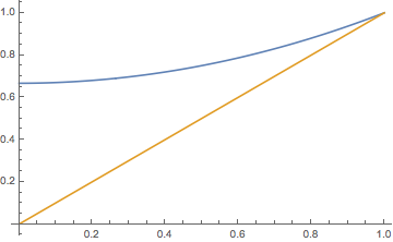
Figure \(\PageIndex{1}\): Graphs of \( r \mapsto \Psi(r) \) and \( r \mapsto r \) when \( p = \frac{1}{3} \)
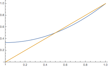
Figure \(\PageIndex{2}\): Graphs of \( r \mapsto \Psi(r) \) and \( r \mapsto r \) when \( p = \frac{2}{3} \)
For \( t \in [0, \infty) \), the generating function \( \Phi_t \) is given by \begin{align*} \Phi_t(r) & = \frac{p r - (1 - p) + (1 - p)(1 - r) e^{\alpha(2 p - 1) t}}{p r - (1 - p) + p(1 - r) e^{\alpha(2 p - 1) t}}, \quad \text{if } p \ne 1/2 \\ \Phi_t(r) & = \frac{2 r + (1 - r) \alpha t}{2 + (1 - r) \alpha t}, \quad \text{if } p = \frac{1}{2} \end{align*}
Solution
The integral equation for \( \Phi_t \) is \[ \int_r^{\Phi_t(r)} \frac{du}{p u^2 + (1 - p) - u} = \alpha t \] The denominator in the integral factors into \( (u - 1)[p u - (1 - p)] \). If \( p \ne \frac{1}{2} \), use partial fractions, standard integration, and some algebra. If \( p = \frac{1}{2} \) the factoring is \( \frac{1}{2}(u - 1)^2 \) and partial fractions is not necessary. Again, use standard integration and algebra.