13.11: Optimal Strategies
- Page ID
- 10456
\( \newcommand{\vecs}[1]{\overset { \scriptstyle \rightharpoonup} {\mathbf{#1}} } \)
\( \newcommand{\vecd}[1]{\overset{-\!-\!\rightharpoonup}{\vphantom{a}\smash {#1}}} \)
\( \newcommand{\id}{\mathrm{id}}\) \( \newcommand{\Span}{\mathrm{span}}\)
( \newcommand{\kernel}{\mathrm{null}\,}\) \( \newcommand{\range}{\mathrm{range}\,}\)
\( \newcommand{\RealPart}{\mathrm{Re}}\) \( \newcommand{\ImaginaryPart}{\mathrm{Im}}\)
\( \newcommand{\Argument}{\mathrm{Arg}}\) \( \newcommand{\norm}[1]{\| #1 \|}\)
\( \newcommand{\inner}[2]{\langle #1, #2 \rangle}\)
\( \newcommand{\Span}{\mathrm{span}}\)
\( \newcommand{\id}{\mathrm{id}}\)
\( \newcommand{\Span}{\mathrm{span}}\)
\( \newcommand{\kernel}{\mathrm{null}\,}\)
\( \newcommand{\range}{\mathrm{range}\,}\)
\( \newcommand{\RealPart}{\mathrm{Re}}\)
\( \newcommand{\ImaginaryPart}{\mathrm{Im}}\)
\( \newcommand{\Argument}{\mathrm{Arg}}\)
\( \newcommand{\norm}[1]{\| #1 \|}\)
\( \newcommand{\inner}[2]{\langle #1, #2 \rangle}\)
\( \newcommand{\Span}{\mathrm{span}}\) \( \newcommand{\AA}{\unicode[.8,0]{x212B}}\)
\( \newcommand{\vectorA}[1]{\vec{#1}} % arrow\)
\( \newcommand{\vectorAt}[1]{\vec{\text{#1}}} % arrow\)
\( \newcommand{\vectorB}[1]{\overset { \scriptstyle \rightharpoonup} {\mathbf{#1}} } \)
\( \newcommand{\vectorC}[1]{\textbf{#1}} \)
\( \newcommand{\vectorD}[1]{\overrightarrow{#1}} \)
\( \newcommand{\vectorDt}[1]{\overrightarrow{\text{#1}}} \)
\( \newcommand{\vectE}[1]{\overset{-\!-\!\rightharpoonup}{\vphantom{a}\smash{\mathbf {#1}}}} \)
\( \newcommand{\vecs}[1]{\overset { \scriptstyle \rightharpoonup} {\mathbf{#1}} } \)
\( \newcommand{\vecd}[1]{\overset{-\!-\!\rightharpoonup}{\vphantom{a}\smash {#1}}} \)
\(\newcommand{\avec}{\mathbf a}\) \(\newcommand{\bvec}{\mathbf b}\) \(\newcommand{\cvec}{\mathbf c}\) \(\newcommand{\dvec}{\mathbf d}\) \(\newcommand{\dtil}{\widetilde{\mathbf d}}\) \(\newcommand{\evec}{\mathbf e}\) \(\newcommand{\fvec}{\mathbf f}\) \(\newcommand{\nvec}{\mathbf n}\) \(\newcommand{\pvec}{\mathbf p}\) \(\newcommand{\qvec}{\mathbf q}\) \(\newcommand{\svec}{\mathbf s}\) \(\newcommand{\tvec}{\mathbf t}\) \(\newcommand{\uvec}{\mathbf u}\) \(\newcommand{\vvec}{\mathbf v}\) \(\newcommand{\wvec}{\mathbf w}\) \(\newcommand{\xvec}{\mathbf x}\) \(\newcommand{\yvec}{\mathbf y}\) \(\newcommand{\zvec}{\mathbf z}\) \(\newcommand{\rvec}{\mathbf r}\) \(\newcommand{\mvec}{\mathbf m}\) \(\newcommand{\zerovec}{\mathbf 0}\) \(\newcommand{\onevec}{\mathbf 1}\) \(\newcommand{\real}{\mathbb R}\) \(\newcommand{\twovec}[2]{\left[\begin{array}{r}#1 \\ #2 \end{array}\right]}\) \(\newcommand{\ctwovec}[2]{\left[\begin{array}{c}#1 \\ #2 \end{array}\right]}\) \(\newcommand{\threevec}[3]{\left[\begin{array}{r}#1 \\ #2 \\ #3 \end{array}\right]}\) \(\newcommand{\cthreevec}[3]{\left[\begin{array}{c}#1 \\ #2 \\ #3 \end{array}\right]}\) \(\newcommand{\fourvec}[4]{\left[\begin{array}{r}#1 \\ #2 \\ #3 \\ #4 \end{array}\right]}\) \(\newcommand{\cfourvec}[4]{\left[\begin{array}{c}#1 \\ #2 \\ #3 \\ #4 \end{array}\right]}\) \(\newcommand{\fivevec}[5]{\left[\begin{array}{r}#1 \\ #2 \\ #3 \\ #4 \\ #5 \\ \end{array}\right]}\) \(\newcommand{\cfivevec}[5]{\left[\begin{array}{c}#1 \\ #2 \\ #3 \\ #4 \\ #5 \\ \end{array}\right]}\) \(\newcommand{\mattwo}[4]{\left[\begin{array}{rr}#1 \amp #2 \\ #3 \amp #4 \\ \end{array}\right]}\) \(\newcommand{\laspan}[1]{\text{Span}\{#1\}}\) \(\newcommand{\bcal}{\cal B}\) \(\newcommand{\ccal}{\cal C}\) \(\newcommand{\scal}{\cal S}\) \(\newcommand{\wcal}{\cal W}\) \(\newcommand{\ecal}{\cal E}\) \(\newcommand{\coords}[2]{\left\{#1\right\}_{#2}}\) \(\newcommand{\gray}[1]{\color{gray}{#1}}\) \(\newcommand{\lgray}[1]{\color{lightgray}{#1}}\) \(\newcommand{\rank}{\operatorname{rank}}\) \(\newcommand{\row}{\text{Row}}\) \(\newcommand{\col}{\text{Col}}\) \(\renewcommand{\row}{\text{Row}}\) \(\newcommand{\nul}{\text{Nul}}\) \(\newcommand{\var}{\text{Var}}\) \(\newcommand{\corr}{\text{corr}}\) \(\newcommand{\len}[1]{\left|#1\right|}\) \(\newcommand{\bbar}{\overline{\bvec}}\) \(\newcommand{\bhat}{\widehat{\bvec}}\) \(\newcommand{\bperp}{\bvec^\perp}\) \(\newcommand{\xhat}{\widehat{\xvec}}\) \(\newcommand{\vhat}{\widehat{\vvec}}\) \(\newcommand{\uhat}{\widehat{\uvec}}\) \(\newcommand{\what}{\widehat{\wvec}}\) \(\newcommand{\Sighat}{\widehat{\Sigma}}\) \(\newcommand{\lt}{<}\) \(\newcommand{\gt}{>}\) \(\newcommand{\amp}{&}\) \(\definecolor{fillinmathshade}{gray}{0.9}\)Basic Theory
Definitions
Recall that the stopping rule for red and black is to continue playing until the gambler is ruined or her fortune reaches the target fortune \(a\). Thus, the gambler's strategy is to decide how much to bet on each game before she must stop. Suppose that we have a class of strategies that correspond to certain valid fortunes and bets; \(A\) will denote the set of fortunes and \(B_x\) will denote the set of valid bets for \(x \in A\). For example, sometimes (as with timid play) we might want to restrict the fortunes to set of integers \(\{0, 1, \ldots, a\}\); other times (as with bold play) we might want to use the interval \([0, 1]\) as the fortune space. As for the bets, recall that the gambler cannot bet what she does not have and will not bet more than she needs in order to reach the target. Thus, a betting function \(S\) must satisfy \[ S(x) \le \min\{x, a - x\}, \quad x \in A \] Moreover, we always restrict our strategies to those for which the stopping time \(N\) is finite.
The success function of a strategy is the probability that the gambler reaches the target \(a\) with that strategy, as a function of the initial fortune \(x\). A strategy with success function \(V\) is optimal if for any other strategy with success function \(U\), we have \(U(x) \le V(x)\) for \(x \in A\).
If there exists an optimal strategy, then the optimal success function is unique.
However, there may not exist an optimal strategy or there may be several optimal strategies. Moreover, the optimality question depends on the value of the game win probability \(p\), in addition to the structure of fortunes and bets.
A Condition for Optimality
Our main theorem gives a condition for optimality:
A strategy \(S\) with success function \(V\) is optimal if \[ p V(x + y) + q V(x - y) \le V(x); \quad x \in A, \, y \in B_x \]
Proof
Consider the following strategy: if the initial fortune is \(x \in A\), we pick \(y \in A_x\) and then bet \(y\) on the first game; thereafter we follow strategy \(S\). Conditioning on the outcome of the first game, the success function for this new strategy is \[ U(x) = p\,V(x + y) + q\,V(x - y) \] Thus, the theorem can be restated as follows: If \(S\) is optimal with respect to the class of strategies just described, then \(S\) is optimal over all strategies. Let \(T\) be an arbitrary strategy with success function \(U\). The random variable \(V(X_n)\) can be interpreted as the probability of winning if the gambler's strategy is replaced by strategy \(S\) after time \(n\). Conditioning on the outcome of game \(n\) gives \[ \E[V(X_n) \mid X_0 = x] = \E[p \, V(X_{n-1} + Y_n) + q \, V(X_{n-1} - Y_n) \mid X_0 = x] \] Using the the optimality condition gives \[ \E[V(X_n) \mid X_0 = x] \le \E[V(X_{n-1}) \mid X_0 = x] , \quad n \in \N_+, \; x \in A \] If follows that \(\E[V(X_n) \mid X_0 = x] \le V(x)\) for \(n \in \N_+\) and \(x \in A\). Now let \(N\) denote the stopping time for strategy \(T\). Letting \(n \to \infty\) we have \(\E[V(X_N) \mid X_0 = x] \le V(x)\) for \(x \in A\). But \(\E[V(X_N) \mid X_0 = x] = U(x)\) for \(x \in A\). Thus \(U(x) \le V(x)\) for \(x \in A\).
Favorable Trials with a Minimum Bet
Suppose now that \(p \ge \frac{1}{2}\) so that the trials are favorable (or at least not unfair) to the gambler. Next, suppose that all bets must be multiples of a basic unit, which we might as well assume is $1. Of course, real gambling houses have this restriction. Thus the set of valid fortunes is \(A = \{0, 1, \ldots, a\}\) and the set of valid bets for \(x \in A\) is \(B_x = \{0, 1, \ldots, \min\{x, a - x\}\}\). Our main result for this case is
Timid play is an optimal strategy.
Proof
Recall the success function \(f\) for timid play and recall the optimality condition. This condition holds if \(p = \frac{1}{2}\). If \(p \gt \frac{1}{2}\), the condition for optimality is equivalent to \[ p \left(\frac{q}{p}\right)^{x+y} + q \left(\frac{q}{p}\right)^{x-y} \ge \left(\frac{q}{p}\right)^x \] But this condition is equivalent to \(p q \left(p^y - q^y\right)\left(p^{y - 1} - q^{y - 1}\right) \le 0\) which clearly holds if \(p \gt \frac{1}{2}\).
In the red and black game set the target fortune to 16, the initial fortune to 8, and the game win probability to 0.45. Define the strategy of your choice and play 100 games. Compare your relative frequency of wins with the probability of winning with timid play.
Favorable Trials without a Minimum Bet
We will now assume that the house allows arbitrarily small bets and that \(p \gt \frac{1}{2}\), so that the trials are strictly favorable. In this case it is natural to take the target as the monetary unit so that the set of fortunes is \(A = [0, 1]\), and the set of bets for \(x \in A\) is \(B_x = [0, \min\{x, 1 - x\}]\). Our main result for this case is given below. The results for timid play will play an important role in the analysis, so we will let \(f(j, a)\) denote the probability of reaching an integer target \(a\), starting at the integer \(j \in [0, a]\), with unit bets.
The optimal success function is \(V(x) = x\) for \(x \in (0, 1]\).
Proof
Fix a rational initial fortune \(x = \frac{k}{n} \in [0, 1]\). Let \(m\) be a positive integer and suppose that, starting at \(x\), the gambler bets \(\frac{1}{m n}\) on each game. This strategy is equivalent to timid play with target fortune \(m n\), and initial fortune \(m k\). Hence the probability of reaching the target 1 under this strategy is \(f(m k, m n)\). But \(f(m k, m n) \to 1\) as \(m \to \infty\). It follows that \(V(x) = x\) if \(x \in (0, 1]\) is rational. But \(V\) is increasing so \(V(x) = x\) for all \(x \in (0, 1]\)
Unfair Trials
We will now assume that \(p \le \frac{1}{2}\) so that the trials are unfair, or at least not favorable. As before, we will take the target fortune as the basic monetary unit and allow any valid fraction of this unit as a bet. Thus, the set of fortunes is \(A = [0, 1]\), and the set of bets for \(x \in A\) is \(B_x = [0, \min\{x, 1 - x\}]\). Our main result for this case is
Bold play is optimal.
Proof
Let \(F\) denote the success function for bold play, and let \[ D(x, y) = F \left(\frac{x + y}{2}\right) - [p F(x) + q F(y)] \] The optimality condition equivalent to \(D(x, y) \le 0\) for \(0 \le x \le y \le 1\). From the continuity of \(F\), it suffices to prove this inequality when \(x\) and \(y\) are binary rationals. It's simple to see that \(D(x, y) \le 0\) when \(x\) and \(y\) have rank 0: \(x = 0\), \(y = 0\) or \(x = 0\), \(y = 1\) or \(x = 1\), \(y = 1\). Suppose now that \(D(x, y) \le 0\) when \(x\) and \(y\) have rank \(m\) or less. We have the following cases:
- If \(x \le y \le \frac{1}{2}\) then \(D(x, y) = p D(2 x, 2 y)\).
- If \(\frac{1}{2} \le x \le y\) then \(D(x, y) = q D(2 x - 1, 2 y - 1)\).
- If \(x \le \frac{x + y}{2} \le \frac{1}{2} \le y\) and \(2 y - 1 \le 2 x\) then \(D(x, y) = (q - p) F(2 y - 1) + q D(2 y - 1, 2 x)\).
- If \(x \le \frac{x + y}{2} \le \frac{1}{2} \le y\) and \(2 x \le 2 y - 1\) then \(D(x, y) = (q - p) F(2 x) + q D(2 x, 2 y - 1)\).
- If \(x \le \frac{1}{2} \le \frac{x + y}{2} \le y\) and \(2 y - 1 \le 2 x\) then \(D(x, y) = p (q - p) [1 - F(2 x)] + p D(2 y - 1, 2 x)\).
- If \(x \le \frac{1}{2} \le \frac{x + y}{2} \le y\) and \(2 x \le 2 y - 1\) then \(D(x, y) = p (q - p) [1 - F(2 y - 1)] + p D(2 x, 2 y - 1)\).
The induction hypothesis can now be applied to each case to finish the proof.
In the red and black game, set the target fortune to 16, the initial fortune to 8, and the game win probability to 0.45. Define the strategy of your choice and play 100 games. Compare your relative frequency of wins with the probability of winning with bold play.
Other Optimal Strategies in the Sub-Fair Case
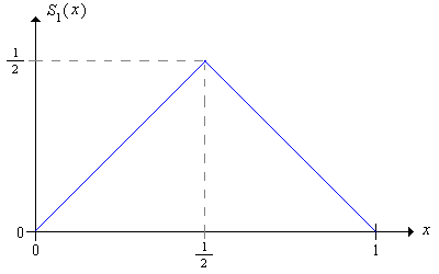
Consider again the sub-fair case where \(p \le \frac{1}{2}\) so that the trials are not favorable to the gambler. We will show that bold play is not the only optimal strategy; amazingly, there are infinitely many optimal strategies. Recall first that the bold strategy has betting function \[ S_1(x) = \min\{x, 1 - x\} = \begin{cases} x, & 0 \le x \le \frac{1}{2} \\ 1 - x, & \frac{1}{2} \le x \le 1 \end{cases} \]

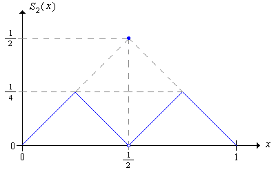
Consider the following strategy, which we will refer to as the second order bold strategy:
- With fortune \(x \in \left(0, \frac{1}{2}\right)\), play boldly with the object of reaching \(\frac{1}{2}\) before falling to 0.
- With fortune \(x \in \left(\frac{1}{2}, 1\right)\), play boldly with the object of reaching 1 without falling below \(\frac{1}{2}\).
- With fortune \(\frac{1}{2}\), play boldly and bet \(\frac{1}{2}\)
The second order bold strategy has betting function \(S_2\) given by \[ S_2(x) = \begin{cases} x, & 0 \le x \lt \frac{1}{4} \\ \frac{1}{2} - x, & \frac{1}{4} \le x \lt \frac{1}{2} \\ \frac{1}{2}, & x = \frac{1}{2} \\ x - \frac{1}{2}, & \frac{1}{2} \lt x \le \frac{3}{4} \\ 1 - x, & \frac{3}{4} \lt x \le 1 \end{cases} \]

The second order bold strategy is optimal.
Proof
Let \(F_2\) denote the success function associated with strategy \(S_2\). Suppose first that the player starts with fortune \(x \in (0, \frac{1}{2})\) under strategy \(S_2\). Note that the player reaches the target 1 if and only if she reaches \(\frac{1}{2}\) and then wins the final game. Consider the sequence of fortunes until the player reaches 0 or \(\frac{1}{2}\). If we double the fortunes, then we have the fortune sequence under the ordinary bold strategy, starting at \(2\,x\) and terminating at either 0 or 1. Thus it follows that \[ F_2(x) = p F(2 x), \quad 0 \lt x \lt \frac{1}{2} \] Suppose next that the player starts with fortune \(x \in (\frac{1}{2}, 1)\) under strategy \(S_2\). Note that the player reaches the target 1 if and only if she reaches 1 without falling back to \(\frac{1}{2}\) or falls back to \(\frac{1}{2}\) and then wins the final game. Consider the sequence of fortunes until the player reaches \(\frac{1}{2}\) or 1. If we double the fortunes and subtract 1, then we have the fortune sequence under the ordinary bold strategy, starting at \(2 x - 1\) and terminating at either 0 or 1. Thus it follows that \[ F_2(x) = F(2 x - 1) + [1 - F(2 x - 2)] p = p + q F(2 x - 1), \quad \frac{1}{2} \lt x \lt 1 \] But now, using the functional equation for ordinary bold play, we have \(F_2(x) = F(x)\) for all \(x \in (0, 1]\), and hence \(S_2\) is optimal.
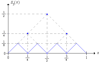
Once we understand how this construction is done, it's straightforward to define the third order bold strategy and show that it's optimal as well.

Explicitly give the third order betting function and show that the strategy is optimal.
More generally, we can define the \(n\)th order bold strategy and show that it is optimal as well.
The sequence of bold strategies can be defined recursively from the basic bold strategy \(S_1\) as follows:
\[ S_{n+1}(x) = \begin{cases} \frac{1}{2} S_n(2 x), & 0 \le x \lt \frac{1}{2} \\ \frac{1}{2}, & x = \frac{1}{2} \\ \frac{1}{2} S_n(2 x - 1), & \frac{1}{2} \lt x \le 1 \end{cases} \]\(S_n\) is optimal for each \(n\).
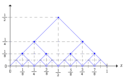
Even more generally, we can define an optimal strategy \(T\) in the following way: for each \(x \in [0, 1]\) select \(n_x \in \N_+\) and let \(T(x) = S_{n_x}(x)\). The graph below shows a few of the graphs of the bold strategies. For an optimal strategy \(T\), we just need to select, for each \(x\) a bet on one of the graphs.

Martingales
Let's return to the unscaled formulation of red and black, where the target fortune is \( a \in (0, \infty) \) and the initial fortune is \( x \in (0, a) \). In the subfair case, when \( p \le \frac{1}{2} \), no strategy can do better than the optimal strategies, so that the win probability is bounded by \( x / a \) (with equality when \( p = \frac{1}{2} \)). Another elegant proof of this is given in the section on inequalities in the chapter on martingales.


