
13.4: Craps
- Page ID
- 10258

\( \newcommand{\vecs}[1]{\overset { \scriptstyle \rightharpoonup} {\mathbf{#1}} } \)
\( \newcommand{\vecd}[1]{\overset{-\!-\!\rightharpoonup}{\vphantom{a}\smash {#1}}} \)
\( \newcommand{\id}{\mathrm{id}}\) \( \newcommand{\Span}{\mathrm{span}}\)
( \newcommand{\kernel}{\mathrm{null}\,}\) \( \newcommand{\range}{\mathrm{range}\,}\)
\( \newcommand{\RealPart}{\mathrm{Re}}\) \( \newcommand{\ImaginaryPart}{\mathrm{Im}}\)
\( \newcommand{\Argument}{\mathrm{Arg}}\) \( \newcommand{\norm}[1]{\| #1 \|}\)
\( \newcommand{\inner}[2]{\langle #1, #2 \rangle}\)
\( \newcommand{\Span}{\mathrm{span}}\)
\( \newcommand{\id}{\mathrm{id}}\)
\( \newcommand{\Span}{\mathrm{span}}\)
\( \newcommand{\kernel}{\mathrm{null}\,}\)
\( \newcommand{\range}{\mathrm{range}\,}\)
\( \newcommand{\RealPart}{\mathrm{Re}}\)
\( \newcommand{\ImaginaryPart}{\mathrm{Im}}\)
\( \newcommand{\Argument}{\mathrm{Arg}}\)
\( \newcommand{\norm}[1]{\| #1 \|}\)
\( \newcommand{\inner}[2]{\langle #1, #2 \rangle}\)
\( \newcommand{\Span}{\mathrm{span}}\) \( \newcommand{\AA}{\unicode[.8,0]{x212B}}\)
\( \newcommand{\vectorA}[1]{\vec{#1}} % arrow\)
\( \newcommand{\vectorAt}[1]{\vec{\text{#1}}} % arrow\)
\( \newcommand{\vectorB}[1]{\overset { \scriptstyle \rightharpoonup} {\mathbf{#1}} } \)
\( \newcommand{\vectorC}[1]{\textbf{#1}} \)
\( \newcommand{\vectorD}[1]{\overrightarrow{#1}} \)
\( \newcommand{\vectorDt}[1]{\overrightarrow{\text{#1}}} \)
\( \newcommand{\vectE}[1]{\overset{-\!-\!\rightharpoonup}{\vphantom{a}\smash{\mathbf {#1}}}} \)
\( \newcommand{\vecs}[1]{\overset { \scriptstyle \rightharpoonup} {\mathbf{#1}} } \)
\( \newcommand{\vecd}[1]{\overset{-\!-\!\rightharpoonup}{\vphantom{a}\smash {#1}}} \)
\(\newcommand{\avec}{\mathbf a}\) \(\newcommand{\bvec}{\mathbf b}\) \(\newcommand{\cvec}{\mathbf c}\) \(\newcommand{\dvec}{\mathbf d}\) \(\newcommand{\dtil}{\widetilde{\mathbf d}}\) \(\newcommand{\evec}{\mathbf e}\) \(\newcommand{\fvec}{\mathbf f}\) \(\newcommand{\nvec}{\mathbf n}\) \(\newcommand{\pvec}{\mathbf p}\) \(\newcommand{\qvec}{\mathbf q}\) \(\newcommand{\svec}{\mathbf s}\) \(\newcommand{\tvec}{\mathbf t}\) \(\newcommand{\uvec}{\mathbf u}\) \(\newcommand{\vvec}{\mathbf v}\) \(\newcommand{\wvec}{\mathbf w}\) \(\newcommand{\xvec}{\mathbf x}\) \(\newcommand{\yvec}{\mathbf y}\) \(\newcommand{\zvec}{\mathbf z}\) \(\newcommand{\rvec}{\mathbf r}\) \(\newcommand{\mvec}{\mathbf m}\) \(\newcommand{\zerovec}{\mathbf 0}\) \(\newcommand{\onevec}{\mathbf 1}\) \(\newcommand{\real}{\mathbb R}\) \(\newcommand{\twovec}[2]{\left[\begin{array}{r}#1 \\ #2 \end{array}\right]}\) \(\newcommand{\ctwovec}[2]{\left[\begin{array}{c}#1 \\ #2 \end{array}\right]}\) \(\newcommand{\threevec}[3]{\left[\begin{array}{r}#1 \\ #2 \\ #3 \end{array}\right]}\) \(\newcommand{\cthreevec}[3]{\left[\begin{array}{c}#1 \\ #2 \\ #3 \end{array}\right]}\) \(\newcommand{\fourvec}[4]{\left[\begin{array}{r}#1 \\ #2 \\ #3 \\ #4 \end{array}\right]}\) \(\newcommand{\cfourvec}[4]{\left[\begin{array}{c}#1 \\ #2 \\ #3 \\ #4 \end{array}\right]}\) \(\newcommand{\fivevec}[5]{\left[\begin{array}{r}#1 \\ #2 \\ #3 \\ #4 \\ #5 \\ \end{array}\right]}\) \(\newcommand{\cfivevec}[5]{\left[\begin{array}{c}#1 \\ #2 \\ #3 \\ #4 \\ #5 \\ \end{array}\right]}\) \(\newcommand{\mattwo}[4]{\left[\begin{array}{rr}#1 \amp #2 \\ #3 \amp #4 \\ \end{array}\right]}\) \(\newcommand{\laspan}[1]{\text{Span}\{#1\}}\) \(\newcommand{\bcal}{\cal B}\) \(\newcommand{\ccal}{\cal C}\) \(\newcommand{\scal}{\cal S}\) \(\newcommand{\wcal}{\cal W}\) \(\newcommand{\ecal}{\cal E}\) \(\newcommand{\coords}[2]{\left\{#1\right\}_{#2}}\) \(\newcommand{\gray}[1]{\color{gray}{#1}}\) \(\newcommand{\lgray}[1]{\color{lightgray}{#1}}\) \(\newcommand{\rank}{\operatorname{rank}}\) \(\newcommand{\row}{\text{Row}}\) \(\newcommand{\col}{\text{Col}}\) \(\renewcommand{\row}{\text{Row}}\) \(\newcommand{\nul}{\text{Nul}}\) \(\newcommand{\var}{\text{Var}}\) \(\newcommand{\corr}{\text{corr}}\) \(\newcommand{\len}[1]{\left|#1\right|}\) \(\newcommand{\bbar}{\overline{\bvec}}\) \(\newcommand{\bhat}{\widehat{\bvec}}\) \(\newcommand{\bperp}{\bvec^\perp}\) \(\newcommand{\xhat}{\widehat{\xvec}}\) \(\newcommand{\vhat}{\widehat{\vvec}}\) \(\newcommand{\uhat}{\widehat{\uvec}}\) \(\newcommand{\what}{\widehat{\wvec}}\) \(\newcommand{\Sighat}{\widehat{\Sigma}}\) \(\newcommand{\lt}{<}\) \(\newcommand{\gt}{>}\) \(\newcommand{\amp}{&}\) \(\definecolor{fillinmathshade}{gray}{0.9}\)The Basic Game
Craps is a popular casino game, because of its complexity and because of the rich variety of bets that can be made.
According to Richard Epstein, craps is descended from an earlier game known as Hazard, that dates to the Middle Ages. The formal rules for Hazard were established by Montmort early in the 1700s. The origin of the name craps is shrouded in doubt, but it may have come from the English crabs or from the French Crapeaud (for toad).
From a mathematical point of view, craps is interesting because it is an example of a random experiment that takes place in stages; the evolution of the game depends critically on the outcome of the first roll. In particular, the number of rolls is a random variable.
Definitions
The rules for craps are as follows:
The player (known as the shooter) rolls a pair of fair dice
- If the sum is 7 or 11 on the first throw, the shooter wins; this event is called a natural.
- If the sum is 2, 3, or 12 on the first throw, the shooter loses; this event is called craps.
- If the sum is 4, 5, 6, 8, 9, or 10 on the first throw, this number becomes the shooter's point. The shooter continues rolling the dice until either she rolls the point again (in which case she wins) or rolls a 7 (in which case she loses).
As long as the shooter wins, or loses by rolling craps, she retrains the dice and continues. Once she loses by failing to make her point, the dice are passed to the next shooter.
Let us consider the game of craps mathematically. Our basic assumption, of course, is that the dice are fair and that the outcomes of the various rolls are independent. Let \(N\) denote the (random) number of rolls in the game and let \((X_i, Y_i)\) denote the outcome of the \(i\)th roll for \(i \in \{1, 2, \ldots, N\}\). Finally, let \(Z_i = X_i + Y_i\), the sum of the scores on the \(i\)th roll, and let \(V\) denote the event that the shooter wins.
In the craps experiment, press single step a few times and observe the outcomes. Make sure that you understand the rules of the game.
The Probability of Winning
We will compute the probability that the shooter wins in stages, based on the outcome of the first roll.
The sum of the scores \(Z\) on a given roll has the probability density function in the following table:
| \(z\) | 2 | 3 | 4 | 5 | 6 | 7 | 8 | 9 | 10 | 11 | 12 |
|---|---|---|---|---|---|---|---|---|---|---|---|
| \(\P(Z = z)\) | \(\frac{1}{36}\) | \(\frac{2}{36}\) | \(\frac{3}{36}\) | \(\frac{4}{36}\) | \(\frac{5}{36}\) | \(\frac{6}{36}\) | \(\frac{5}{36}\) | \(\frac{4}{36}\) | \(\frac{3}{36}\) | \(\frac{2}{36}\) | \(\frac{1}{36}\) |
The probability that the player makes her point can be computed using a simple conditioning argument. For example, suppose that the player throws 4 initially, so that 4 is the point. The player continues until she either throws 4 again or throws 7. Thus, the final roll will be an element of the following set: \[ S_4 = \{(1,3), (2,2), (3,1), (1,6), (2,5), (3,4), (4,3), (5,2), (6,1)\} \] Since the dice are fair, these outcomes are equally likely, so the probability that the player makes her 4 point is \(\frac{3}{9}\). A similar argument can be used for the other points. Here are the results:
The probabilities of making the point \(z\) are given in the following table:
| \(z\) | 4 | 5 | 6 | 8 | 9 | 10 |
|---|---|---|---|---|---|---|
| \(\P(V \mid Z_1 = z)\) | \(\frac{3}{9}\) | \(\frac{4}{10}\) | \(\frac{5}{11}\) | \(\frac{5}{11}\) | \(\frac{4}{10}\) | \(\frac{3}{9}\) |
The probability that the shooter wins is \(\P(V) = \frac{244}{495} \approx 0.49293\)
Proof
This follows from the the rules of the game and the the previous result, by conditioning on the first roll:
\[ \P(V) = \sum_{z=2}^{12} \P(Z_1 = z) \P(I = 1 \mid Z_1 = z) \]Note that craps is nearly a fair game. For the sake of completeness, the following result gives the probability of winning, given a point
on the first roll.
\( \P(V \mid Z_1 \in \{4, 5, 6, 8, 9, 10\}) = \frac{67}{165} \approx 0.406 \)
Proof
Let \( A = \{4, 5, 6, 8, 9, 10\} \). From the definition of conditional probability, \[ \P(V \mid Z_1 \in A) = \frac{\P(V \cap \{Z_1 \in A\})}{\P(Z_1 \in A)} \] For the numerator, using our results above, \[ \P(V \cap \{Z_1 \in A\}) = \sum_{z \in A} \P(V \mid Z_1 = z) \P(Z_1 = z) = \frac{134}{495} \] Also from previous results \( \P(Z_1 \in A) = \frac{2}{3} \).
Bets
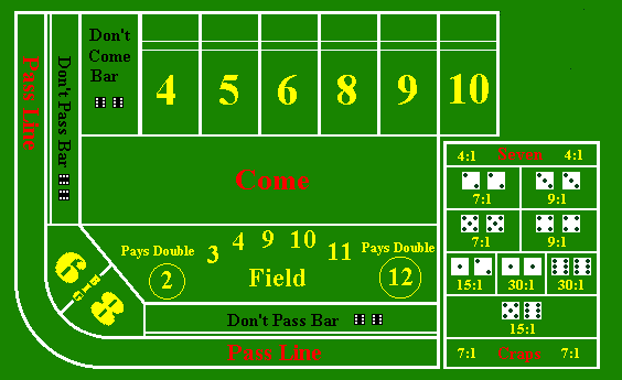
There is a bewildering variety of bets that can be made in craps. In the exercises in this subsection, we will discuss some typical bets and compute the probability density function, mean, and standard deviation of each. (Most of these bets are illustrated in the picture of the craps table above). Note however, that some of the details of the bets and, in particular the payout odds, vary from one casino to another. Of course the expected value of any bet is inevitably negative (for the gambler), and thus the gambler is doomed to lose money in the long run. Nonetheless, as we will see, some bets are better than others.
Pass and Don't Pass
A pass bet is a bet that the shooter will win and pays \(1 : 1\).
Let \(W\) denote the winnings from a unit pass bet. Then
- \(\P(W = -1) = \frac{251}{495}\), \(\P(W = 1) = \frac{244}{495}\)
- \(\E(W) = -\frac{7}{495} \approx -0.0141\)
- \(\sd(W) \approx 0.9999\)
In the craps experiment, select the pass bet. Run the simulation 1000 times and compare the empirical density function and moments of \(W\) to the true probability density function and moments. Suppose that you bet $1 on each of the 1000 games. What would your net winnings be?
A don't pass bet is a bet that the shooter will lose, except that 12 on the first throw is excluded (that is, the shooter loses, of course, but the don't pass better neither wins nor loses). This is the meaning of the phrase don't pass bar double 6 on the craps table. The don't pass bet also pays \(1 : 1\).
Let \(W\) denote the winnings for a unit don't pass bet. Then
- \(\P(W = -1) = \frac{244}{495}\), \(\P(W = 0) = \frac{1}{36}\), \(\P(W = 1) = \frac{949}{1980}\)
- \(\E(W) = -\frac{27}{1980} \approx -0.01363\)
- \(\sd(W) \approx 0.9859\)
Thus, the don't pass bet is slightly better for the gambler than the pass bet.
In the craps experiment, select the don't pass bet. Run the simulation 1000 times and compare the empirical density function and moments of \(W\) to the true probability density function and moments. Suppose that you bet $1 on each of the 1000 games. What would your net winnings be?
The come bet and the don't come bet are analogous to the pass and don't pass bets, respectively, except that they are made after the point has been established.
Field
A field bet is a bet on the outcome of the next throw. It pays \(1 : 1\) if 3, 4, 9, 10, or 11 is thrown, \(2 : 1\) if 2 or 12 is thrown, and loses otherwise.
Let \(W\) denote the winnings for a unit field bet. Then
- \(\P(W = -1) = \frac{5}{9}\), \(\P(W = 1) = \frac{7}{18}\), \(\P(W = 2) = \frac{1}{18}\)
- \(\E(W) = -\frac{1}{18} \approx -0.0556\)
- \(\sd(W) \approx 1.0787\)
In the craps experiment, select the field bet. Run the simulation 1000 times and compare the empirical density function and moments of \(W\) to the true probability density function and moments. Suppose that you bet $1 on each of the 1000 games. What would your net winnings be?
Seven and Eleven
A 7 bet is a bet on the outcome of the next throw. It pays \(4 : 1\) if a 7 is thrown. Similarly, an 11 bet is a bet on the outcome of the next throw, and pays \(15 : 1\) if an 11 is thrown. In spite of the romance of the number 7, the next exercise shows that the 7 bet is one of the worst bets you can make.
Let \(W\) denote the winnings for a unit 7 bet. Then
- \(\P(W = -1) = \frac{5}{6}\), \(\P(W = 4) = \frac{1}{6}\)
- \(\E(W) = -\frac{1}{6} \approx -0.1667\)
- \(\sd(W) \approx 1.8634\)
In the craps experiment, select the 7 bet. Run the simulation 1000 times and compare the empirical density function and moments of \(W\) to the true probability density function and moments. Suppose that you bet $1 on each of the 1000 games. What would your net winnings be?
Let \(W\) denote the winnings for a unit 11 bet. Then
- \(\P(W = -1) = \frac{17}{18}\), \(\P(W = 15) = \frac{1}{18}\)
- \(\E(W) = -\frac{1}{9} \approx -0.1111\)
- \(\sd(W) \approx 3.6650\)
In the craps experiment, select the 11 bet. Run the simulation 1000 times and compare the empirical density function and moments of \(W\) to the true probability density function and moments. Suppose that you bet $1 on each of the 1000 games. What would your net winnings be?
Craps
All craps bets are bets on the next throw. The basic craps bet pays \(7 : 1\) if 2, 3, or 12 is thrown. The craps 2 bet pays \(30 : 1\) if a 2 is thrown. Similarly, the craps 12 bet pays \(30 : 1\) if a 12 is thrown. Finally, the craps 3 bet pays \(15 : 1\) if a 3 is thrown.
Let \(W\) denote the winnings for a unit craps bet. Then
- \(\P(W = -1) = \frac{8}{9}\), \(\P(W = 7) = \frac{1}{9}\)
- \(\E(W) = -\frac{1}{9} \approx -0.1111\)
- \(\sd(W) \approx 5.0944\)
In the craps experiment, select the craps bet. Run the simulation 1000 times and compare the empirical density function and moments of \(W\) to the true probability density function and moments. Suppose that you bet $1 on each of the 1000 games. What would your net winnings be?
Let \(W\) denote the winnings for a unit craps 2 bet or a unit craps 12 bet. Then
- \(\P(W = -1) = \frac{35}{36}\), \(\P(W = 30) = \frac{1}{36}\)
- \(\E(W) = -\frac{5}{36} \approx -0.1389\)
- \(\sd(W) = 5.0944\)
In the craps experiment, select the craps 2 bet. Run the simulation 1000 times and compare the empirical density function and moments of \(W\) to the true probability density function and moments. Suppose that you bet $1 on each of the 1000 games. What would your net winnings be?
In the craps experiment, select the craps 12 bet. Run the simulation 1000 times and compare the empirical density function and moments of \(W\) to the true probability density function and moments. Suppose that you bet $1 on each of the 1000 games. What would your net winnings be?
Let \(W\) denote the winnings for a unit craps 3 bet. Then
- \(\P(W = -1) = \frac{17}{18}\), \( \P(W = 15) = \frac{1}{18} \)
- \(\E(W) = -\frac{1}{9} \approx -0.1111\)
- \(\sd(W) \approx 3.6650\)
In the craps experiment, select the craps 3 bet. Run the simulation 1000 times and compare the empirical density function and moments of \(W\) to the true probability density function and moments. Suppose that you bet $1 on each of the 1000 games. What would your net winnings be?
Thus, of the craps bets, the basic craps bet and the craps 3 bet are best for the gambler, and the craps 2 and craps 12 are the worst.
Big Six and Big Eight
The big 6 bet is a bet that 6 is thrown before 7. Similarly, the big 8 bet is a bet that 8 is thrown before 7. Both pay even money \(1 : 1\).
Let \(W\) denote the winnings for a unit big 6 bet or a unit big 8 bet. Then
- \(\P(W = -1) = \frac{6}{11}\), \(\P(W = 1) = \frac{5}{11}\)
- \(\E(W) = -\frac{1}{11} \approx -0.0909\)
- \(\sd(W) \approx 0.9959\)
In the craps experiment, select the big 6 bet. Run the simulation 1000 times and compare the empirical density function and moments of \(W\) to the true probability density function and moments. Suppose that you bet $1 on each of the 1000 games. What would your net winnings be?
In the craps experiment, select the big 8 bet. Run the simulation 1000 times and compare the empirical density function and moments of \(W\) to the true probability density function and moments. Suppose that you bet $1 on each of the 1000 games. What would your net winnings be?
Hardway Bets
A hardway bet can be made on any of the numbers 4, 6, 8, or 10. It is a bet that the chosen number \(n\) will be thrown the hardway
as \( (n/2, n/2) \), before 7 is thrown and before the chosen number is thrown in any other combination. Hardway bets on 4 and 10 pay \(7 : 1\), while hardway bets on 6 and 8 pay \(9 : 1\).
Let \(W\) denote the winnings for a unit hardway 4 or hardway 10 bet. Then
- \(\P(W = -1) = \frac{8}{9}\), \(\P(W = 7) = \frac{1}{9}\)
- \(\E(W) = -\frac{1}{9} \approx -0.1111\)
- \(\sd(W) = 2.5142\)
In the craps experiment, select the hardway 4 bet. Run the simulation 1000 times and compare the empirical density function and moments of \(W\) to the true probability density function and moments. Suppose that you bet $1 on each of the 1000 games. What would your net winnings be?
In the craps experiment, select the hardway 10 bet. Run the simulation 1000 times and compare the empirical density function and moments of \(W\) to the true probability density function and moments. Suppose that you bet $1 on each of the 1000 games. What would your net winnings be?
Let \(W\) denote the winnings for a unit hardway 6 or hardway 8 bet. Then
- \(\P(W = -1) = \frac{10}{11}\), \(\P(W = 9) = \frac{1}{11}\)
- \(\E(W) = -\frac{1}{11} \approx -0.0909\)
- \(\sd(W) \approx 2.8748\)
In the craps experiment, select the hardway 6 bet. Run the simulation 1000 times and compare the empirical density and moments of \(W\) to the true density and moments. Suppose that you bet $1 on each of the 1000 games. What would your net winnings be?
In the craps experiment, select the hardway 8 bet. Run the simulation 1000 times and compare the empirical density function and moments of \(W\) to the true probability density function and moments. Suppose that you bet $1 on each of the 1000 games. What would your net winnings be?
Thus, the hardway 6 and 8 bets are better than the hardway 4 and 10 bets for the gambler, in terms of expected value.
The Distribution of the Number of Rolls
Next let us compute the distribution and moments of the number of rolls \(N\) in a game of craps. This random variable is of no special interest to the casino or the players, but provides a good mathematically exercise. By definition, if the shooter wins or loses on the first roll, \(N = 1\). Otherwise, the shooter continues until she either makes her point or rolls 7. In this latter case, we can use the geometric distribution on \(\N_+\) which governs the trial number of the first success in a sequence of Bernoulli trials. The distribution of \(N\) is a mixture of distributions.
The probability density function of \(N\) is
\[ \P(N = n) = \begin{cases} \frac{12}{36}, & n = 1 \\ \frac{1}{24} \left(\frac{3}{4}\right)^{n-2} + \frac{5}{81} \left(\frac{13}{18}\right)^{n-2} + \frac{55}{648} \left(\frac{25}{36}\right)^{n-2}, & n \in \{2, 3, \ldots\} \end{cases} \]Proof
First note that \(\P(N = 1 \mid Z_1 = z) = 1\) for \(z \in \{2, 3, 7, 11, 12\}\). Next, \(\P(N = n \mid Z_1 = z) = p_z (1 - p_z)^{n-2}\) for \(n \in \{2, 3, \ldots\}\) and for the values of \(z\) and \(p_z\) given in the following table:
| \(z\) | 4 | 5 | 6 | 8 | 9 | 10 |
|---|---|---|---|---|---|---|
| \(p_z\) | \(\frac{9}{36}\) | \(\frac{10}{36}\) | \(\frac{11}{36}\) | \(\frac{11}{36}\) | \(\frac{10}{36}\) | \(\frac{9}{36}\) |
Thus the conditional distribution of \(N - 1\) given \(Z = z\) is geometric with probability \(p_z\). The final result now follows by conditioning on the first roll: \[ \P(N = n) = \sum_{z=2}^{12} \P(Z_1 = z) \P(N = n \mid Z_1 = z) \]
The first few values of the probability density function of \(N\) are given in the following table:
| \(n\) | 1 | 2 | 3 | 4 | 5 |
|---|---|---|---|---|---|
| \(\P(N = n)\) | 0.33333 | 0.18827 | 0.13477 | 0.09657 | 0.06926 |
Find the probability that a game of craps will last at least 8 rolls.
Answer
0.09235
The mean and variance of the number of rolls are
- \(\E(N) = \frac{557}{165} \approx 3.3758\)
- \(\var(N) = \frac{245\,672}{27\,225} \approx 9.02376\)
Proof
These result also can be obtained by conditioning on the first roll: \begin{align} \E(N) & = \E\left[\E(N \mid Z_1)\right] = \frac{557}{165} \\ \E(N^2) & = \E\left[\E\left(N^2 \mid Z_1\right)\right] = \frac{61\,769}{3025} \end{align}