
13.1: Introduction to Games of Chance
- Page ID
- 10255

\( \newcommand{\vecs}[1]{\overset { \scriptstyle \rightharpoonup} {\mathbf{#1}} } \)
\( \newcommand{\vecd}[1]{\overset{-\!-\!\rightharpoonup}{\vphantom{a}\smash {#1}}} \)
\( \newcommand{\id}{\mathrm{id}}\) \( \newcommand{\Span}{\mathrm{span}}\)
( \newcommand{\kernel}{\mathrm{null}\,}\) \( \newcommand{\range}{\mathrm{range}\,}\)
\( \newcommand{\RealPart}{\mathrm{Re}}\) \( \newcommand{\ImaginaryPart}{\mathrm{Im}}\)
\( \newcommand{\Argument}{\mathrm{Arg}}\) \( \newcommand{\norm}[1]{\| #1 \|}\)
\( \newcommand{\inner}[2]{\langle #1, #2 \rangle}\)
\( \newcommand{\Span}{\mathrm{span}}\)
\( \newcommand{\id}{\mathrm{id}}\)
\( \newcommand{\Span}{\mathrm{span}}\)
\( \newcommand{\kernel}{\mathrm{null}\,}\)
\( \newcommand{\range}{\mathrm{range}\,}\)
\( \newcommand{\RealPart}{\mathrm{Re}}\)
\( \newcommand{\ImaginaryPart}{\mathrm{Im}}\)
\( \newcommand{\Argument}{\mathrm{Arg}}\)
\( \newcommand{\norm}[1]{\| #1 \|}\)
\( \newcommand{\inner}[2]{\langle #1, #2 \rangle}\)
\( \newcommand{\Span}{\mathrm{span}}\) \( \newcommand{\AA}{\unicode[.8,0]{x212B}}\)
\( \newcommand{\vectorA}[1]{\vec{#1}} % arrow\)
\( \newcommand{\vectorAt}[1]{\vec{\text{#1}}} % arrow\)
\( \newcommand{\vectorB}[1]{\overset { \scriptstyle \rightharpoonup} {\mathbf{#1}} } \)
\( \newcommand{\vectorC}[1]{\textbf{#1}} \)
\( \newcommand{\vectorD}[1]{\overrightarrow{#1}} \)
\( \newcommand{\vectorDt}[1]{\overrightarrow{\text{#1}}} \)
\( \newcommand{\vectE}[1]{\overset{-\!-\!\rightharpoonup}{\vphantom{a}\smash{\mathbf {#1}}}} \)
\( \newcommand{\vecs}[1]{\overset { \scriptstyle \rightharpoonup} {\mathbf{#1}} } \)
\( \newcommand{\vecd}[1]{\overset{-\!-\!\rightharpoonup}{\vphantom{a}\smash {#1}}} \)
\(\newcommand{\avec}{\mathbf a}\) \(\newcommand{\bvec}{\mathbf b}\) \(\newcommand{\cvec}{\mathbf c}\) \(\newcommand{\dvec}{\mathbf d}\) \(\newcommand{\dtil}{\widetilde{\mathbf d}}\) \(\newcommand{\evec}{\mathbf e}\) \(\newcommand{\fvec}{\mathbf f}\) \(\newcommand{\nvec}{\mathbf n}\) \(\newcommand{\pvec}{\mathbf p}\) \(\newcommand{\qvec}{\mathbf q}\) \(\newcommand{\svec}{\mathbf s}\) \(\newcommand{\tvec}{\mathbf t}\) \(\newcommand{\uvec}{\mathbf u}\) \(\newcommand{\vvec}{\mathbf v}\) \(\newcommand{\wvec}{\mathbf w}\) \(\newcommand{\xvec}{\mathbf x}\) \(\newcommand{\yvec}{\mathbf y}\) \(\newcommand{\zvec}{\mathbf z}\) \(\newcommand{\rvec}{\mathbf r}\) \(\newcommand{\mvec}{\mathbf m}\) \(\newcommand{\zerovec}{\mathbf 0}\) \(\newcommand{\onevec}{\mathbf 1}\) \(\newcommand{\real}{\mathbb R}\) \(\newcommand{\twovec}[2]{\left[\begin{array}{r}#1 \\ #2 \end{array}\right]}\) \(\newcommand{\ctwovec}[2]{\left[\begin{array}{c}#1 \\ #2 \end{array}\right]}\) \(\newcommand{\threevec}[3]{\left[\begin{array}{r}#1 \\ #2 \\ #3 \end{array}\right]}\) \(\newcommand{\cthreevec}[3]{\left[\begin{array}{c}#1 \\ #2 \\ #3 \end{array}\right]}\) \(\newcommand{\fourvec}[4]{\left[\begin{array}{r}#1 \\ #2 \\ #3 \\ #4 \end{array}\right]}\) \(\newcommand{\cfourvec}[4]{\left[\begin{array}{c}#1 \\ #2 \\ #3 \\ #4 \end{array}\right]}\) \(\newcommand{\fivevec}[5]{\left[\begin{array}{r}#1 \\ #2 \\ #3 \\ #4 \\ #5 \\ \end{array}\right]}\) \(\newcommand{\cfivevec}[5]{\left[\begin{array}{c}#1 \\ #2 \\ #3 \\ #4 \\ #5 \\ \end{array}\right]}\) \(\newcommand{\mattwo}[4]{\left[\begin{array}{rr}#1 \amp #2 \\ #3 \amp #4 \\ \end{array}\right]}\) \(\newcommand{\laspan}[1]{\text{Span}\{#1\}}\) \(\newcommand{\bcal}{\cal B}\) \(\newcommand{\ccal}{\cal C}\) \(\newcommand{\scal}{\cal S}\) \(\newcommand{\wcal}{\cal W}\) \(\newcommand{\ecal}{\cal E}\) \(\newcommand{\coords}[2]{\left\{#1\right\}_{#2}}\) \(\newcommand{\gray}[1]{\color{gray}{#1}}\) \(\newcommand{\lgray}[1]{\color{lightgray}{#1}}\) \(\newcommand{\rank}{\operatorname{rank}}\) \(\newcommand{\row}{\text{Row}}\) \(\newcommand{\col}{\text{Col}}\) \(\renewcommand{\row}{\text{Row}}\) \(\newcommand{\nul}{\text{Nul}}\) \(\newcommand{\var}{\text{Var}}\) \(\newcommand{\corr}{\text{corr}}\) \(\newcommand{\len}[1]{\left|#1\right|}\) \(\newcommand{\bbar}{\overline{\bvec}}\) \(\newcommand{\bhat}{\widehat{\bvec}}\) \(\newcommand{\bperp}{\bvec^\perp}\) \(\newcommand{\xhat}{\widehat{\xvec}}\) \(\newcommand{\vhat}{\widehat{\vvec}}\) \(\newcommand{\uhat}{\widehat{\uvec}}\) \(\newcommand{\what}{\widehat{\wvec}}\) \(\newcommand{\Sighat}{\widehat{\Sigma}}\) \(\newcommand{\lt}{<}\) \(\newcommand{\gt}{>}\) \(\newcommand{\amp}{&}\) \(\definecolor{fillinmathshade}{gray}{0.9}\)Gambling and Probability
Games of chance are among the oldest of human inventions. The use of a certain type of animal heel bone (called the astragalus or colloquially the knucklebone) as a crude die dates to about 3600 BCE. The modern six-sided die dates to 2000 BCE, and the term bones is used as a slang expression for dice to this day (as in roll the bones). It is because of these ancient origins, by the way, that we use the die as the fundamental symbol in this project.
Gambling is intimately interwoven with the development of probability as a mathematical theory. Most of the early development of probability, in particular, was stimulated by special gambling problems, such as
- DeMere's problem
- Pepy's problem
- the problem of points
- the Petersburg problem
Some of the very first books on probability theory were written to analyze games of chance, for example Liber de Ludo Aleae (The Book on Games of Chance), by Girolamo Cardano, and Essay d' Analyse sur les Jeux de Hazard (Analytical Essay on Games of Chance), by Pierre-Remond Montmort. Gambling problems continue to be a source of interesting and deep problems in probability to this day (see the discussion of Red and Black for an example).
Of course, it is important to keep in mind that breakthroughs in probability, even when they are originally motivated by gambling problems, are often profoundly important in the natural sciences, the social sciences, law, and medicine. Also, games of chance provide some of the conceptually clearest and cleanest examples of random experiments, and thus their analysis can be very helpful to students of probability.
However, nothing in this chapter should be construed as encouraging you, gentle reader, to gamble. On the contrary, our analysis will show that, in the long run, only the gambling houses prosper. The gambler, inevitably, is a sad victim of the law of large numbers.
In this chapter we will study some interesting games of chance. Poker, poker dice, craps, and roulette are popular parlor and casino games. The Monty Hall problem, on the other hand, is interesting because of the controversy that it generated. The lottery is a basic way that many states and nations use to raise money (a voluntary tax, of sorts).
Terminology
Let us discuss some of the basic terminology that will be used in several sections of this chapter. Suppose that \(A\) is an event in a random experiment. The mathematical odds concerning \(A\) refer to the probability of \(A\).
If \(a\) and \(b\) are positive numbers, then by definition, the following are equivalent:
- the odds in favor of \(A\) are \(a : b\).
- \(\P(A) = \frac{a}{a + b}\).
- the odds against \(A\) are \(b : a\).
- \(\P(A^c) = \frac{b}{a + b}\).
In many cases, \(a\) and \(b\) can be given as positive integers with no common factors.
Similarly, suppose that \(p \in [0, 1]\). The following are equivalent:
- \(\P(A) = p\).
- The odds in favor of \(A\) are \(p : 1 - p\).
- \(\P(A^c) = 1 - p\).
- The odds against \(A\) are \(1 - p : p\).
On the other hand, the house odds of an event refer to the payout when a bet is made on the event.
A bet on event \(A\) pays \(n : m\) means that if a gambler bets \( m \) units on \( A \) then
- If \(A\) occurs, the gambler receives the \(m\) units back and an additional \(n\) units (for a net profit of \(n\))
- If \(A\) does not occur, the gambler loses the bet of \(m\) units (for a net profit of \(-m\)).
Equivalently, the gambler puts up \(m\) units (betting on \(A\)), the house puts up \(n\) units, (betting on \(A^c\)) and the winner takes the pot. Of course, it is usually not necessary for the gambler to bet exactly \(m\); a smaller or larger is bet is scaled appropriately. Thus, if the gambler bets \(k\) units and wins, his payout is \(k \frac{n}{m}\).
Naturally, our main interest is in the net winnings if we make a bet on an event. The following result gives the probability density function, mean, and variance for a unit bet. The expected value is particularly interesting, because by the law of large numbers, it gives the long term gain or loss, per unit bet.
Suppose that the odds in favor of event \(A\) are \(a : b\) and that a bet on event \(A\) pays \(n : m\). Let \(W\) denote the winnings from a unit bet on \(A\). Then
- \(\P(W = -1) = \frac{b}{a + b}\), \(\P\left(W = \frac{n}{m}\right) = \frac{a}{a + b}\)
- \(\E(W) = \frac{a\,n - b m}{m(a + b)}\)
- \(\var(W) = \frac{a b (n + m)^2}{m^2 (a + b)^2}\)
In particular, the expected value of the bet is zero if and only if \(a n = b m\), positive if and only if \(a n \gt b m\), and negative if and only if \(a n \lt b m\). The first case means that the bet is fair, and occurs when the payoff is the same as the odds against the event. The second means that the bet is favorable to the gambler, and occurs when the payoff is greater that the odds against the event. The third case means that the bet is unfair to the gambler, and occurs when the payoff is less than the odds against the event. Unfortunately, all casino games fall into the third category.
More About Dice
Shapes of Dice
The standard die, of course, is a cube with six sides. A bit more generally, most real dice are in the shape of Platonic solids, named for Plato naturally. The faces of a Platonic solid are congruent regular polygons. Moreover, the same number of faces meet at each vertex so all of the edges and angles are congruent as well.
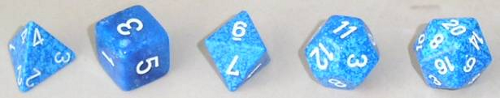
The five Platonic solids are
- The tetrahedron, with 4 sides.
- The hexahedron (cube), with 6 sides
- The octahedron, with 8 sides
- The dodecahedron, with 12 sides
- The icosahedron, with 20 sides
Note that the 4-sided die is the only Platonic die in which the outcome is the face that is down rather than up (or perhaps it's better to think of the vertex that is up as the outcome).
Fair and Crooked Dice
Recall that a fair die is one in which the faces are equally likely. In addition to fair dice, there are various types of crooked dice. For the standard six-sided die, there are three crooked types that we use frequently in this project. To understand the geometry, recall that with the standard six-sided die, opposite faces sum to 7.
Flat Dice
- An ace-six flat die is a six-sided die in which faces 1 and 6 have probability \(\frac{1}{4}\) each while faces 2, 3, 4, and 5 have probability \(\frac{1}{8}\) each.
- A two-five flat die is a six-sided die in which faces 2 and 5 have probability \(\frac{1}{4}\) each while faces 1, 3, 4, and 6 have probability \(\frac{1}{8}\) each.
- A three-four flat die is a six-sided die in which faces 3 and 4 have probability \(\frac{1}{4}\) each while faces 1, 2, 5, and 6 have probability \(\frac{1}{8}\) each.
A flat die, as the name suggests, is a die that is not a cube, but rather is shorter in one of the three directions. The particular probabilities that we use (\(1/4\) and \(1/8\)) are fictitious, but the essential property of a flat die is that the opposite faces on the shorter axis have slightly larger probabilities (because they have slightly larger areas) than the other four faces. Flat dice are sometimes used by gamblers to cheat.
In the Dice Experiment, select one die. Run the experiment 1000 times in each of the following cases and observe the outcomes.
- fair die
- ace-six flat die
- two-five flat die
- three-four flat die
Simulation
It's very easy to simulate a fair die with a random number. Recall that the ceiling function \(\lceil x \rceil\) gives the smallest integer that is at least as large as \(x\).
Suppose that \(U\) is uniformly distributed on the interval \((0, 1]\), so that \(U\) has the standard uniform distribution (a random number). Then \(X = \lceil 6 \, U \rceil\) is uniformly distributed on the set \(\{1, 2, 3, 4, 5, 6\}\) and so simulates a fair six-sided die. More generally, \(X = \lceil n \, U \rceil\) is uniformly distributed on \(\{1, 2, \ldots, n\}\) and so simlates a fair \(n\)-sided die.
We can also use a real fair die to simulate other types of fair dice. Recall that if \(X\) is uniformly distributed on \(\{1, 2, \ldots, n\}\) and \(k \in \{1, 2, \ldots, n - 1\}\), then the conditional distribution of \(X\) given that \(X \in \{1, 2, \ldots, k\}\) is uniformly distributed on \(\{1, 2, \ldots, k\}\). Thus, suppose that we have a real, fair, \(n\)-sided die. If we ignore outcomes greater than \(k\) then we simulate a fair \(k\)-sided die. For example, suppose that we have a carefully constructed icosahedron that is a fair 20-sided die. We can simulate a fair 13-sided die by simply rolling the die and stopping as soon as we have a score between 1 and 13.
To see how to simulate a card hand, see the Introduction to Finite Sampling Models. A general method of simulating random variables is based on the quantile function.