
11.1: Introduction
- Page ID
- 3172

\( \newcommand{\vecs}[1]{\overset { \scriptstyle \rightharpoonup} {\mathbf{#1}} } \)
\( \newcommand{\vecd}[1]{\overset{-\!-\!\rightharpoonup}{\vphantom{a}\smash {#1}}} \)
\( \newcommand{\id}{\mathrm{id}}\) \( \newcommand{\Span}{\mathrm{span}}\)
( \newcommand{\kernel}{\mathrm{null}\,}\) \( \newcommand{\range}{\mathrm{range}\,}\)
\( \newcommand{\RealPart}{\mathrm{Re}}\) \( \newcommand{\ImaginaryPart}{\mathrm{Im}}\)
\( \newcommand{\Argument}{\mathrm{Arg}}\) \( \newcommand{\norm}[1]{\| #1 \|}\)
\( \newcommand{\inner}[2]{\langle #1, #2 \rangle}\)
\( \newcommand{\Span}{\mathrm{span}}\)
\( \newcommand{\id}{\mathrm{id}}\)
\( \newcommand{\Span}{\mathrm{span}}\)
\( \newcommand{\kernel}{\mathrm{null}\,}\)
\( \newcommand{\range}{\mathrm{range}\,}\)
\( \newcommand{\RealPart}{\mathrm{Re}}\)
\( \newcommand{\ImaginaryPart}{\mathrm{Im}}\)
\( \newcommand{\Argument}{\mathrm{Arg}}\)
\( \newcommand{\norm}[1]{\| #1 \|}\)
\( \newcommand{\inner}[2]{\langle #1, #2 \rangle}\)
\( \newcommand{\Span}{\mathrm{span}}\) \( \newcommand{\AA}{\unicode[.8,0]{x212B}}\)
\( \newcommand{\vectorA}[1]{\vec{#1}} % arrow\)
\( \newcommand{\vectorAt}[1]{\vec{\text{#1}}} % arrow\)
\( \newcommand{\vectorB}[1]{\overset { \scriptstyle \rightharpoonup} {\mathbf{#1}} } \)
\( \newcommand{\vectorC}[1]{\textbf{#1}} \)
\( \newcommand{\vectorD}[1]{\overrightarrow{#1}} \)
\( \newcommand{\vectorDt}[1]{\overrightarrow{\text{#1}}} \)
\( \newcommand{\vectE}[1]{\overset{-\!-\!\rightharpoonup}{\vphantom{a}\smash{\mathbf {#1}}}} \)
\( \newcommand{\vecs}[1]{\overset { \scriptstyle \rightharpoonup} {\mathbf{#1}} } \)
\( \newcommand{\vecd}[1]{\overset{-\!-\!\rightharpoonup}{\vphantom{a}\smash {#1}}} \)
\(\newcommand{\avec}{\mathbf a}\) \(\newcommand{\bvec}{\mathbf b}\) \(\newcommand{\cvec}{\mathbf c}\) \(\newcommand{\dvec}{\mathbf d}\) \(\newcommand{\dtil}{\widetilde{\mathbf d}}\) \(\newcommand{\evec}{\mathbf e}\) \(\newcommand{\fvec}{\mathbf f}\) \(\newcommand{\nvec}{\mathbf n}\) \(\newcommand{\pvec}{\mathbf p}\) \(\newcommand{\qvec}{\mathbf q}\) \(\newcommand{\svec}{\mathbf s}\) \(\newcommand{\tvec}{\mathbf t}\) \(\newcommand{\uvec}{\mathbf u}\) \(\newcommand{\vvec}{\mathbf v}\) \(\newcommand{\wvec}{\mathbf w}\) \(\newcommand{\xvec}{\mathbf x}\) \(\newcommand{\yvec}{\mathbf y}\) \(\newcommand{\zvec}{\mathbf z}\) \(\newcommand{\rvec}{\mathbf r}\) \(\newcommand{\mvec}{\mathbf m}\) \(\newcommand{\zerovec}{\mathbf 0}\) \(\newcommand{\onevec}{\mathbf 1}\) \(\newcommand{\real}{\mathbb R}\) \(\newcommand{\twovec}[2]{\left[\begin{array}{r}#1 \\ #2 \end{array}\right]}\) \(\newcommand{\ctwovec}[2]{\left[\begin{array}{c}#1 \\ #2 \end{array}\right]}\) \(\newcommand{\threevec}[3]{\left[\begin{array}{r}#1 \\ #2 \\ #3 \end{array}\right]}\) \(\newcommand{\cthreevec}[3]{\left[\begin{array}{c}#1 \\ #2 \\ #3 \end{array}\right]}\) \(\newcommand{\fourvec}[4]{\left[\begin{array}{r}#1 \\ #2 \\ #3 \\ #4 \end{array}\right]}\) \(\newcommand{\cfourvec}[4]{\left[\begin{array}{c}#1 \\ #2 \\ #3 \\ #4 \end{array}\right]}\) \(\newcommand{\fivevec}[5]{\left[\begin{array}{r}#1 \\ #2 \\ #3 \\ #4 \\ #5 \\ \end{array}\right]}\) \(\newcommand{\cfivevec}[5]{\left[\begin{array}{c}#1 \\ #2 \\ #3 \\ #4 \\ #5 \\ \end{array}\right]}\) \(\newcommand{\mattwo}[4]{\left[\begin{array}{rr}#1 \amp #2 \\ #3 \amp #4 \\ \end{array}\right]}\) \(\newcommand{\laspan}[1]{\text{Span}\{#1\}}\) \(\newcommand{\bcal}{\cal B}\) \(\newcommand{\ccal}{\cal C}\) \(\newcommand{\scal}{\cal S}\) \(\newcommand{\wcal}{\cal W}\) \(\newcommand{\ecal}{\cal E}\) \(\newcommand{\coords}[2]{\left\{#1\right\}_{#2}}\) \(\newcommand{\gray}[1]{\color{gray}{#1}}\) \(\newcommand{\lgray}[1]{\color{lightgray}{#1}}\) \(\newcommand{\rank}{\operatorname{rank}}\) \(\newcommand{\row}{\text{Row}}\) \(\newcommand{\col}{\text{Col}}\) \(\renewcommand{\row}{\text{Row}}\) \(\newcommand{\nul}{\text{Nul}}\) \(\newcommand{\var}{\text{Var}}\) \(\newcommand{\corr}{\text{corr}}\) \(\newcommand{\len}[1]{\left|#1\right|}\) \(\newcommand{\bbar}{\overline{\bvec}}\) \(\newcommand{\bhat}{\widehat{\bvec}}\) \(\newcommand{\bperp}{\bvec^\perp}\) \(\newcommand{\xhat}{\widehat{\xvec}}\) \(\newcommand{\vhat}{\widehat{\vvec}}\) \(\newcommand{\uhat}{\widehat{\uvec}}\) \(\newcommand{\what}{\widehat{\wvec}}\) \(\newcommand{\Sighat}{\widehat{\Sigma}}\) \(\newcommand{\lt}{<}\) \(\newcommand{\gt}{>}\) \(\newcommand{\amp}{&}\) \(\definecolor{fillinmathshade}{gray}{0.9}\)Most of our study of probability has dealt with independent trials processes. These processes are the basis of classical probability theory and much of statistics. We have discussed two of the principal theorems for these processes: the Law of Large Numbers and the Central Limit Theorem.
We have seen that when a sequence of chance experiments forms an independent trials process, the possible outcomes for each experiment are the same and occur with the same probability. Further, knowledge of the outcomes of the previous experiments does not influence our predictions for the outcomes of the next experiment. The distribution for the outcomes of a single experiment is sufficient to construct a tree and a tree measure for a sequence of \(n\) experiments, and we can answer any probability question about these experiments by using this tree measure.
Modern probability theory studies chance processes for which the knowledge of previous outcomes influences predictions for future experiments. In principle, when we observe a sequence of chance experiments, all of the past outcomes could influence our predictions for the next experiment. For example, this should be the case in predicting a student’s grades on a sequence of exams in a course. But to allow this much generality would make it very difficult to prove general results.
In 1907, A. A. Markov began the study of an important new type of chance process. In this process, the outcome of a given experiment can affect the outcome of the next experiment. This type of process is called a Markov chain.
Specifying a Markov Chain
According to Kemeny, Snell, and Thompson, \({ }^2\) the Land of \(\mathrm{Oz}\) is blessed by many things, but not by good weather. They never have two nice days in a row. If they have a nice day, they are just as likely to have snow as rain the next day. If they have snow or rain, they have an even chance of having the same the next day. If there is change from snow or rain, only half of the time is this a change to a nice day. With this information we form a Markov chain as follows. We take as states the kinds of weather R, N, and S. From the above information we determine the transition probabilities. These are most conveniently represented in a square array as
\[P= \begin{matrix}
& \begin{matrix}R&N&S\end{matrix} \\
\begin{matrix}R\\N\\S\end{matrix} &
\begin{pmatrix}1/2 & 1/4 & 1/4 \\1 / 2 & 0 & 1 / 2\\ 1/4 & 1/4 & 1/2\end{pmatrix}\\
\end{matrix}\]
Transition Matrix
The entries in the first row of the matrix \(\mathbf{P}\) in Example 11.1 represent the probabilities for the various kinds of weather following a rainy day. Similarly, the entries in the second and third rows represent the probabilities for the various kinds of weather following nice and snowy days, respectively. Such a square array is called the matrix of transition probabilities, or the transition matrix.
We consider the question of determining the probability that, given the chain is in state \(i\) today, it will be in state \(j\) two days from now. We denote this probability by \(p_{i j}^{(2)}\). In Example \(\PageIndex{1}\), we see that if it is rainy today then the event that it is snowy two days from now is the disjoint union of the following three events: 1) it is rainy tomorrow and snowy two days from now, 2) it is nice tomorrow and snowy two days from now, and 3) it is snowy tomorrow and snowy two days from now. The probability of the first of these events is the product of the conditional probability that it is rainy tomorrow, given that it is rainy today, and the conditional probability that it is snowy two days from now, given that it is rainy tomorrow. Using the transition matrix \(\mathbf{P}\), we can write this product as \(p_{11} p_{13}\). The other two
events also have probabilities that can be written as products of entries of \(\mathbf{P}\). Thus, we have
\[
p_{13}^{(2)}=p_{11} p_{13}+p_{12} p_{23}+p_{13} p_{33} .
\]
This equation should remind the reader of a dot product of two vectors; we are dotting the first row of \(\mathbf{P}\) with the third column of \(\mathbf{P}\). This is just what is done in obtaining the 1,3-entry of the product of \(\mathbf{P}\) with itself. In general, if a Markov chain has \(r\) states, then
\[
p_{i j}^{(2)}=\sum_{k=1}^r p_{i k} p_{k j} .
\]
The following general theorem is easy to prove by using the above observation and induction.
Let \(\mathbf{P}\) be the transition matrix of a Markov chain. The \(i j\) th entry \(p_{i j}^{(n)}\) of the matrix \(\mathbf{P}^n\) gives the probability that the Markov chain, starting in state \(s_i\), will be in state \(s_j\) after \(n\) steps.
Proof. The proof of this theorem is left as an exercise (Exercise \(\PageIndex{17}\)).
(Example \(\PageIndex{1}\) continued) Consider again the weather in the Land of \(\mathrm{Oz}\). We know that the powers of the transition matrix give us interesting information about the process as it evolves. We shall be particularly interested in the state of the chain after a large number of steps. The program MatrixPowers computes the powers of \(\mathbf{P}\).
We have run the program MatrixPowers for the Land of \(\mathrm{Oz}\) example to compute the successive powers of \(\mathbf{P}\) from 1 to 6 . The results are shown in Table \(\PageIndex{1}\). We note that after six days our weather predictions are, to three-decimal-place accuracy, independent of today's weather. The probabilities for the three types of weather, \(\mathrm{R}, \mathrm{N}\), and \(\mathrm{S}\), are \(.4, .2\), and .4 no matter where the chain started. This is an example of a type of Markov chain called a regular Markov chain. For this type of chain, it is true that long-range predictions are independent of the starting state. Not all chains are regular, but this is an important class of chains that we shall study in detail later.
We now consider the long-term behavior of a Markov chain when it starts in a state chosen by a probability distribution on the set of states, which we will call a probability vector. A probability vector with \(r\) components is a row vector whose entries are non-negative and sum to 1 . If \(\mathbf{u}\) is a probability vector which represents the initial state of a Markov chain, then we think of the \(i\) th component of \(\mathbf{u}\) as representing the probability that the chain starts in state \(s_i\).
With this interpretation of random starting states, it is easy to prove the following theorem.
\[P= \begin{matrix} & \begin{matrix}Rain&Nice&Snow\end{matrix} \\\begin{matrix}Rain\\Nice\\Snow\end{matrix} & \begin{pmatrix}.500 & .250 & .250 \\
.500 & .000 & .500 \\.250 & .250 & .500\end{pmatrix}\\\end{matrix}\]
\[P= \begin{matrix} & \begin{matrix}Rain&Nice&Snow\end{matrix} \\\begin{matrix}Rain\\Nice\\Snow\end{matrix} & \begin{pmatrix}.438 & .188 & .375 \\
.375 & .250 & .375 \\.375 & .188 & .438\end{pmatrix}\\\end{matrix}\]
\[P= \begin{matrix} & \begin{matrix}Rain&Nice&Snow\end{matrix} \\\begin{matrix}Rain\\Nice\\Snow\end{matrix} & \begin{pmatrix}.406 & .203 & .391 \\
.406 & .188 & .406 \\.391 & .203 & .406\end{pmatrix}\\\end{matrix}\]
\[P= \begin{matrix} & \begin{matrix}Rain&Nice&Snow\end{matrix} \\\begin{matrix}Rain\\Nice\\Snow\end{matrix} & \begin{pmatrix}.402 & .199 & .398 \\
.398 & .203 & .398 \\.398 & .199 & .402\end{pmatrix}\\\end{matrix}\]
\[P= \begin{matrix} & \begin{matrix}Rain&Nice&Snow\end{matrix} \\\begin{matrix}Rain\\Nice\\Snow\end{matrix} & \begin{pmatrix}.400 & .200 & .399 \\
.400 & .199 & .400 \\.399 & .200 & .400\end{pmatrix}\\\end{matrix}\]
\[P= \begin{matrix} & \begin{matrix}Rain&Nice&Snow\end{matrix} \\\begin{matrix}Rain\\Nice\\Snow\end{matrix} & \begin{pmatrix}.400 & .200 & .400 \\
.400 & .200 & .400 \\.400 & .200 & .400\end{pmatrix}\\\end{matrix}\]
Table \(\PageIndex{1}\): Powers of the Land of \(\mathrm{Oz}\) transition matrix.
Let \(\mathbf{P}\) be the transition matrix of a Markov chain, and let \(\mathbf{u}\) be the probability vector which represents the starting distribution. Then the probability that the chain is in state \(s_i\) after \(n\) steps is the \(i\) th entry in the vector
\[
\mathbf{u}^{(n)}=\mathbf{u} \mathbf{P}^n
\]
Proof. The proof of this theorem is left as an exercise (Exercise \(\PageIndex{18}\).).
We note that if we want to examine the behavior of the chain under the assumption that it starts in a certain state \(s_i\), we simply choose \(\mathbf{u}\) to be the probability vector with \(i\) th entry equal to 1 and all other entries equal to 0 .
In the Land of Oz example (Example \(\PageIndex{1}\)) let the initial probability vector \(\mathbf{u}\) equal \((1 / 3,1 / 3,1 / 3)\). Then we can calculate the distribution of the states after three days using Theorem \(\PageIndex{2}\). and our previous calculation of \(\mathbf{P}^3\). We obtain
\[
\begin{aligned}
\mathbf{u}^{(3)}=\mathbf{u} \mathbf{P}^3 & =\left(\begin{array}{lll}
1 / 3, & 1 / 3, & 1 / 3
\end{array}\right)\left(\begin{array}{ccc}
.406 & .203 & .391 \\
.406 & .188 & .406 \\
.391 & .203 & .406
\end{array}\right) \\ \\
& =\left(\begin{array}{lll}
.401, & .198, & .401
\end{array}\right) .
\end{aligned}
\]
Examples
The following examples of Markov chains will be used throughout the chapter for exercises.
The President of the United States tells person A his or her intention to run or not to run in the next election. Then A relays the news to B, who in turn relays the message to \(\mathrm{C}\), and so forth, always to some new person. We assume that there is a probability \(a\) that a person will change the answer from yes to no when transmitting it to the next person and a probability \(b\) that he or she will change it from no to yes. We choose as states the message, either yes or no. The transition matrix is then
\[P= \begin{matrix} & \begin{matrix}Yes&No\end{matrix} \\\begin{matrix}Yes\\No\end{matrix} & \begin{pmatrix}1-a & a \\
b & 1-b\end{pmatrix}\\\end{matrix}\]
The initial state represents the President's choice.
Each time a certain horse runs in a three-horse race, he has probability \(1 / 2\) of winning, 1/4 of coming in second, and 1/4 of coming in third, independent of the outcome of any previous race. We have an independent trials process, but it can also be considered from the point of view of Markov chain theory. The transition matrix is
\[P= \begin{matrix} & \begin{matrix}W&P&S\end{matrix} \\\begin{matrix}W\\P\\S\end{matrix} & \begin{pmatrix}.5 & .25&.25\\.5&.25&.25 \\.5&.25 &.25\end{pmatrix}\\\end{matrix}\]
A
In the Dark Ages, Harvard, Dartmouth, and Yale admitted only male students. Assume that, at that time, 80 percent of the sons of Harvard men went to Harvard and the rest went to Yale, 40 percent of the sons of Yale men went to Yale, and the rest split evenly between Harvard and Dartmouth; and of the sons of Dartmouth men, 70 percent went to Dartmouth, 20 percent to Harvard, and 10 percent to Yale. We form a Markov chain with transition matrix
\[P= \begin{matrix} & \begin{matrix}H&Y&D\end{matrix} \\\begin{matrix}H\\Y\\D\end{matrix} & \begin{pmatrix}.8 & .2 & 0 \\.3 & .4 & .3 \\.2 & .1 & .7\end{pmatrix}\\\end{matrix}\]
Modify Example \(\PageIndex{6}\) by assuming that the son of a Harvard man always went to Harvard. The transition matrix is now
\[P= \begin{matrix} & \begin{matrix}H&Y&D\end{matrix} \\\begin{matrix}H\\Y\\D\end{matrix} & \begin{pmatrix}1 & 0 & 0 \\.3 & .4 & .3 \\.2 & .1 & .7\end{pmatrix}\\\end{matrix}\]
(Ehrenfest Model) The following is a special case of a model, called the Ehrenfest model, \({ }^3\) that has been used to explain diffusion of gases. The general model will be discussed in detail in Section 11.5. We have two urns that, between them, contain four balls. At each step, one of the four balls is chosen at random and moved from the urn that it is in into the other urn. We choose, as states, the number of balls in the first urn. The transition matrix is then
\[P= \begin{matrix} & \begin{matrix}0&&1&&2&&3&&4\end{matrix} \\\begin{matrix}0\\1\\2\\3\\4\end{matrix} & \begin{pmatrix}0 & 1 & 0 & 0 & 0 \\1 / 4 & 0 & 3 / 4 & 0 & 0 \\0 & 1 / 2 & 0 & 1 / 2 & 0 \\0 & 0 & 3 / 4 & 0 & 1 / 4 \\0 & 0 & 0 & 1 & 0\end{pmatrix}\\\end{matrix}\]
\({ }^3\) P. and T. Ehrenfest, "Über zwei bekannte Einwände gegen das Boltzmannsche H-Theorem," Physikalishce Zeitschrift, vol. 8 (1907), pp. 311-314.
(Gene Model) The simplest type of inheritance of traits in animals occurs when a trait is governed by a pair of genes, each of which may be of two types, say \(\mathrm{G}\) and \(\mathrm{g}\). An individual may have a GG combination or Gg (which is genetically the same as \(\mathrm{gG}\) ) or gg. Very often the GG and Gg types are indistinguishable in appearance, and then we say that the \(\mathrm{G}\) gene dominates the g gene. An individual is called dominant if he or she has GG genes, recessive if he or she has gg, and hybrid with a Gg mixture.
In the mating of two animals, the offspring inherits one gene of the pair from each parent, and the basic assumption of genetics is that these genes are selected at random, independently of each other. This assumption determines the probability of occurrence of each type of offspring. The offspring of two purely dominant parents must be dominant, of two recessive parents must be recessive, and of one dominant and one recessive parent must be hybrid.
In the mating of a dominant and a hybrid animal, each offspring must get a \(\mathrm{G}\) gene from the former and has an equal chance of getting \(\mathrm{G}\) or \(\mathrm{g}\) from the latter. Hence there is an equal probability for getting a dominant or a hybrid offspring. Again, in the mating of a recessive and a hybrid, there is an even chance for getting either a recessive or a hybrid. In the mating of two hybrids, the offspring has an equal chance of getting \(\mathrm{G}\) or \(\mathrm{g}\) from each parent. Hence the probabilities are \(1 / 4\) for \(\mathrm{GG}, 1 / 2\) for \(\mathrm{Gg}\), and \(1 / 4\) for gg.
Consider a process of continued matings. We start with an individual of known genetic character and mate it with a hybrid. We assume that there is at least one offspring. An offspring is chosen at random and is mated with a hybrid and this process repeated through a number of generations. The genetic type of the chosen offspring in successive generations can be represented by a Markov chain. The states are dominant, hybrid, and recessive, and indicated by GG, Gg, and gg respectively.
The transition probabilities are
\[P= \begin{matrix} & \begin{matrix}GG&Gg&gg\end{matrix} \\\begin{matrix}GG\\Gg\\gg\end{matrix} & \begin{pmatrix}1 & 0 & 0 \\.25 & .5 & .25 \\0 & .5 & .5\end{pmatrix}\\\end{matrix}\]
Modify Example \(\PageIndex{9}\). as follows: Instead of mating the oldest offspring with a hybrid, we mate it with a dominant individual. The transition matrix is
\[P= \begin{matrix} & \begin{matrix}GG&Gg&gg\end{matrix} \\\begin{matrix}GG\\Gg\\gg\end{matrix} & \begin{pmatrix}1 & 0 & 0 \\
.5 & .5 & 0 \\
0 & 1 & 0\end{pmatrix}\\\end{matrix}\]
We start with two animals of opposite sex, mate them, select two of their offspring of opposite sex, and mate those, and so forth. To simplify the example, we will assume that the trait under consideration is independent of sex.
Here a state is determined by a pair of animals. Hence, the states of our process will be:
\[P= \begin{matrix} & \begin{matrix}GG,GG&GG,Gg&GG,gg&Gg,Gg&Gg,gg&gg,gg\end{matrix} \\\begin{matrix}GG,GG\\GG,Gg\\GG,gg\\Gg,Gg\\Gg,gg\\gg,gg\end{matrix} & \begin{pmatrix}1.000 && .000 && .000 && .000 && .000 && .000 \\
.250 && .500 && .000 && .250 && .000 && .000 \\
.000 && .000 &&.000 && 1.000 && .000 && .000 \\
.062 && .250 && .125 && .250 && .250 && .062 \\
.000 && .000 && .000 && .250 && .500 && .250 \\
.000 && .000 && .000 && .000 && .000 && 1.000\end{pmatrix}\\\end{matrix}\]
We illustrate the calculation of transition probabilities in terms of the state \(s_2\). When the process is in this state, one parent has GG genes, the other Gg. Hence, the probability of a dominant offspring is \(1 / 2\). Then the probability of transition to \(s_1\) (selection of two dominants) is \(1 / 4\), transition to \(s_2\) is \(1 / 2\), and to \(s_4\) is \(1 / 4\). The other states are treated the same way. The transition matrix of this chain is:
(Stepping Stone Model) Our final example is another example that has been used in the study of genetics. It is called the stepping stone model. \({ }^4\) In this model we have an \(n\)-by- \(n\) array of squares, and each square is initially any one of \(k\) different colors. For each step, a square is chosen at random. This square then chooses one of its eight neighbors at random and assumes the color of that neighbor. To avoid boundary problems, we assume that if a square \(S\) is on the left-hand boundary, say, but not at a corner, it is adjacent to the square \(T\) on the right-hand boundary in the same row as \(S\), and \(S\) is also adjacent to the squares just above and below \(T\). A similar assumption is made about squares on the upper and lower boundaries. The top left-hand corner square is adjacent to three obvious neighbors, namely the squares below it, to its right, and diagonally below and to the right. It has five other neighbors, which are as follows: the other three corner squares, the square below the upper right-hand corner, and the square to the right of the bottom left-hand corner. The other three corners also have, in a similar way, eight neighbors. (These adjacencies are much easier to understand if one imagines making the array into a cylinder by gluing the top and bottom edge together, and then making the cylinder into a doughnut by gluing the two circular boundaries together.) With these adjacencies, each square in the array is adjacent to exactly eight other squares.
A state in this Markov chain is a description of the color of each square. For this Markov chain the number of states is \(k^{n^2}\), which for even a small array of squares
\({ }^4\) S. Sawyer, "Results for The Stepping Stone Model for Migration in Population Genetics," Annals of Probability, vol. 4 (1979), pp. 699-728.
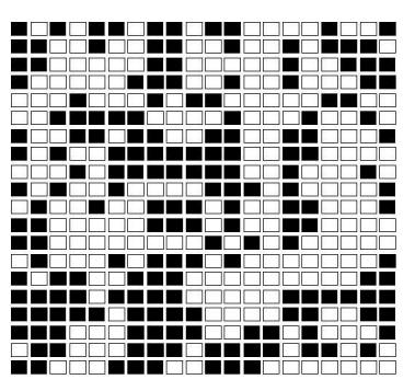

is enormous. This is an example of a Markov chain that is easy to simulate but difficult to analyze in terms of its transition matrix. The program SteppingStone simulates this chain. We have started with a random initial configuration of two colors with \(n=20\) and show the result after the process has run for some time in Figure 1\(\PageIndex{2}\)..
This is an example of an absorbing Markov chain. This type of chain will be studied in Section 11.2. One of the theorems proved in that section, applied to the present example, implies that with probability 1 , the stones will eventually all be the same color. By watching the program run, you can see that territories are established and a battle develops to see which color survives. At any time the probability that a particular color will win out is equal to the proportion of the array of this color. You are asked to prove this in Exercise 11.2.32.
Exercises
Exercise \(\PageIndex{1}\):
It is raining in the Land of \(\mathrm{Oz}\). Determine a tree and a tree measure for the next three days' weather. Find \(\mathbf{w}^{(1)}, \mathbf{w}^{(2)}\), and \(\mathbf{w}^{(3)}\) and compare with the results obtained from \(\mathbf{P}, \mathbf{P}^2\), and \(\mathbf{P}^3\).
Exercise \(\PageIndex{2}\):
In Example (\PageIndex{4}\, let \(a=0\) and \(b=1 / 2\). Find \(\mathbf{P}, \mathbf{P}^2\), and \(\mathbf{P}^3\). What would \(\mathbf{P}^n\) be? What happens to \(\mathbf{P}^n\) as \(n\) tends to infinity? Interpret this result.
Exercise \(\PageIndex{3}\):
In Example (\PageIndex{5}\, find \(\mathbf{P}, \mathbf{P}^2\), and \(\mathbf{P}^3\). What is \(\mathbf{P}^n\) ?
Exercise \(\PageIndex{4}\):
For Example (\PageIndex{6}\, find the probability that the grandson of a man from Harvard went to Harvard.
Exercise \(\PageIndex{5}\):
In Example (\PageIndex{7}\, find the probability that the grandson of a man from Harvard went to Harvard.
Exercise \(\PageIndex{6}\):
In Example (\PageIndex{9}\, assume that we start with a hybrid bred to a hybrid. Find \(\mathbf{u}^{(1)}, \mathbf{u}^{(2)}\), and \(\mathbf{u}^{(3)}\). What would \(\mathbf{u}^{(n)}\) be?
Exercise \(\PageIndex{7}\):
Find the matrices \(\mathbf{P}^2, \mathbf{P}^3, \mathbf{P}^4\), and \(\mathbf{P}^n\) for the Markov chain determined by the transition matrix \(\mathbf{P}=\left(\begin{array}{ll}1 & 0 \\ 0 & 1\end{array}\right)\). Do the same for the transition matrix \(\mathbf{P}=\left(\begin{array}{ll}0 & 1 \\ 1 & 0\end{array}\right)\). Interpret what happens in each of these processes.
Exercise \(\PageIndex{8}\):
A certain calculating machine uses only the digits 0 and 1 . It is supposed to transmit one of these digits through several stages. However, at every stage, there is a probability \(p\) that the digit that enters this stage will be changed when it leaves and a probability \(q=1-p\) that it won't. Form a Markov chain to represent the process of transmission by taking as states the digits 0 and 1 . What is the matrix of transition probabilities?
Exercise \(\PageIndex{9}\):
For the Markov chain in Exercise \(\PageIndex{8}\)., draw a tree and assign a tree measure assuming that the process begins in state 0 and moves through two stages of transmission. What is the probability that the machine, after two stages, produces the digit 0 (i.e., the correct digit)? What is the probability that the machine never changed the digit from 0 ? Now let \(p=.1\). Using the program MatrixPowers, compute the 100th power of the transition matrix. Interpret the entries of this matrix. Repeat this with \(p=.2\). Why do the 100th powers appear to be the same?
Exercise \(\PageIndex{10}\):
Modify the program MatrixPowers so that it prints out the average \(\mathbf{A}_n\) of the powers \(\mathbf{P}^n\), for \(n=1\) to \(N\). Try your program on the Land of \(\mathrm{Oz}\) example and compare \(\mathbf{A}_n\) and \(\mathbf{P}^n\).
Exercise \(\PageIndex{11}\):
Assume that a man's profession can be classified as professional, skilled laborer, or unskilled laborer. Assume that, of the sons of professional men, 80 percent are professional, 10 percent are skilled laborers, and 10 percent are unskilled laborers. In the case of sons of skilled laborers, 60 percent are skilled laborers, 20 percent are professional, and 20 percent are unskilled. Finally, in the case of unskilled laborers, 50 percent of the sons are unskilled laborers, and 25 percent each are in the other two categories. Assume that every man has at least one son, and form a Markov chain by following the profession of a randomly chosen son of a given family through several generations. Set up the matrix of transition probabilities. Find the probability that a randomly chosen grandson of an unskilled laborer is a professional man.
Exercise \(\PageIndex{12}\):
In Exercise (\PageIndex{11}\, we assumed that every man has a son. Assume instead that the probability that a man has at least one son is .8. Form a Markov chain with four states. If a man has a son, the probability that this son is in a particular profession is the same as in Exercise \(\PageIndex{11}\).. If there is no son, the process moves to state four which represents families whose male line has died out. Find the matrix of transition probabilities and find the probability that a randomly chosen grandson of an unskilled laborer is a professional man.
Exercise \(\PageIndex{13}\):
Write a program to compute \(\mathbf{u}^{(n)}\) given \(\mathbf{u}\) and \(\mathbf{P}\). Use this program to compute \(\mathbf{u}^{(10)}\) for the Land of \(\mathrm{Oz}\) example, with \(\mathbf{u}=(0,1,0)\), and with \(\mathbf{u}=(1 / 3,1 / 3,1 / 3)\).
Exercise \(\PageIndex{14}\):
Using the program MatrixPowers, find \(\mathbf{P}^1\) through \(\mathbf{P}^6\) for Examples \(\PageIndex{9}\). and \(\PageIndex{10}\).. See if you can predict the long-range probability of finding the process in each of the states for these examples.
Exercise \(\PageIndex{15}\):
Write a program to simulate the outcomes of a Markov chain after \(n\) steps, given the initial starting state and the transition matrix \(\mathbf{P}\) as data (see Example \(\PageIndex{12}\).). Keep this program for use in later problems.
Exercise \(\PageIndex{16}\):
Modify the program of Exercise (\PageIndex{15}\ so that it keeps track of the proportion of times in each state in \(n\) steps. Run the modified program for different starting states for Example (\PageIndex{1}\ and Example (\PageIndex{8}\. Does the initial state affect the proportion of time spent in each of the states if \(n\) is large?
Exercise \(\PageIndex{17}\):
Prove Theorem \(\PageIndex{1}\).
Exercise \(\PageIndex{18}\):
Prove Theorem \(\PageIndex{2}\).
Exercise \(\PageIndex{19}\):
Consider the following process. We have two coins, one of which is fair, and the other of which has heads on both sides. We give these two coins to our friend, who chooses one of them at random (each with probability \(1 / 2\) ). During the rest of the process, she uses only the coin that she chose. She now proceeds to toss the coin many times, reporting the results. We consider this process to consist solely of what she reports to us.
(a) Given that she reports a head on the \(n\)th toss, what is the probability that a head is thrown on the \((n+1)\) st toss?
(b) Consider this process as having two states, heads and tails. By computing the other three transition probabilities analogous to the one in part (a), write down a "transition matrix" for this process.
(c) Now assume that the process is in state "heads" on both the \((n-1)\) st and the \(n\)th toss. Find the probability that a head comes up on the \((n+1)\) st toss.
(d) Is this process a Markov chain?