
4.3: Paradoxes
- Page ID
- 3137

\( \newcommand{\vecs}[1]{\overset { \scriptstyle \rightharpoonup} {\mathbf{#1}} } \)
\( \newcommand{\vecd}[1]{\overset{-\!-\!\rightharpoonup}{\vphantom{a}\smash {#1}}} \)
\( \newcommand{\dsum}{\displaystyle\sum\limits} \)
\( \newcommand{\dint}{\displaystyle\int\limits} \)
\( \newcommand{\dlim}{\displaystyle\lim\limits} \)
\( \newcommand{\id}{\mathrm{id}}\) \( \newcommand{\Span}{\mathrm{span}}\)
( \newcommand{\kernel}{\mathrm{null}\,}\) \( \newcommand{\range}{\mathrm{range}\,}\)
\( \newcommand{\RealPart}{\mathrm{Re}}\) \( \newcommand{\ImaginaryPart}{\mathrm{Im}}\)
\( \newcommand{\Argument}{\mathrm{Arg}}\) \( \newcommand{\norm}[1]{\| #1 \|}\)
\( \newcommand{\inner}[2]{\langle #1, #2 \rangle}\)
\( \newcommand{\Span}{\mathrm{span}}\)
\( \newcommand{\id}{\mathrm{id}}\)
\( \newcommand{\Span}{\mathrm{span}}\)
\( \newcommand{\kernel}{\mathrm{null}\,}\)
\( \newcommand{\range}{\mathrm{range}\,}\)
\( \newcommand{\RealPart}{\mathrm{Re}}\)
\( \newcommand{\ImaginaryPart}{\mathrm{Im}}\)
\( \newcommand{\Argument}{\mathrm{Arg}}\)
\( \newcommand{\norm}[1]{\| #1 \|}\)
\( \newcommand{\inner}[2]{\langle #1, #2 \rangle}\)
\( \newcommand{\Span}{\mathrm{span}}\) \( \newcommand{\AA}{\unicode[.8,0]{x212B}}\)
\( \newcommand{\vectorA}[1]{\vec{#1}} % arrow\)
\( \newcommand{\vectorAt}[1]{\vec{\text{#1}}} % arrow\)
\( \newcommand{\vectorB}[1]{\overset { \scriptstyle \rightharpoonup} {\mathbf{#1}} } \)
\( \newcommand{\vectorC}[1]{\textbf{#1}} \)
\( \newcommand{\vectorD}[1]{\overrightarrow{#1}} \)
\( \newcommand{\vectorDt}[1]{\overrightarrow{\text{#1}}} \)
\( \newcommand{\vectE}[1]{\overset{-\!-\!\rightharpoonup}{\vphantom{a}\smash{\mathbf {#1}}}} \)
\( \newcommand{\vecs}[1]{\overset { \scriptstyle \rightharpoonup} {\mathbf{#1}} } \)
\(\newcommand{\longvect}{\overrightarrow}\)
\( \newcommand{\vecd}[1]{\overset{-\!-\!\rightharpoonup}{\vphantom{a}\smash {#1}}} \)
\(\newcommand{\avec}{\mathbf a}\) \(\newcommand{\bvec}{\mathbf b}\) \(\newcommand{\cvec}{\mathbf c}\) \(\newcommand{\dvec}{\mathbf d}\) \(\newcommand{\dtil}{\widetilde{\mathbf d}}\) \(\newcommand{\evec}{\mathbf e}\) \(\newcommand{\fvec}{\mathbf f}\) \(\newcommand{\nvec}{\mathbf n}\) \(\newcommand{\pvec}{\mathbf p}\) \(\newcommand{\qvec}{\mathbf q}\) \(\newcommand{\svec}{\mathbf s}\) \(\newcommand{\tvec}{\mathbf t}\) \(\newcommand{\uvec}{\mathbf u}\) \(\newcommand{\vvec}{\mathbf v}\) \(\newcommand{\wvec}{\mathbf w}\) \(\newcommand{\xvec}{\mathbf x}\) \(\newcommand{\yvec}{\mathbf y}\) \(\newcommand{\zvec}{\mathbf z}\) \(\newcommand{\rvec}{\mathbf r}\) \(\newcommand{\mvec}{\mathbf m}\) \(\newcommand{\zerovec}{\mathbf 0}\) \(\newcommand{\onevec}{\mathbf 1}\) \(\newcommand{\real}{\mathbb R}\) \(\newcommand{\twovec}[2]{\left[\begin{array}{r}#1 \\ #2 \end{array}\right]}\) \(\newcommand{\ctwovec}[2]{\left[\begin{array}{c}#1 \\ #2 \end{array}\right]}\) \(\newcommand{\threevec}[3]{\left[\begin{array}{r}#1 \\ #2 \\ #3 \end{array}\right]}\) \(\newcommand{\cthreevec}[3]{\left[\begin{array}{c}#1 \\ #2 \\ #3 \end{array}\right]}\) \(\newcommand{\fourvec}[4]{\left[\begin{array}{r}#1 \\ #2 \\ #3 \\ #4 \end{array}\right]}\) \(\newcommand{\cfourvec}[4]{\left[\begin{array}{c}#1 \\ #2 \\ #3 \\ #4 \end{array}\right]}\) \(\newcommand{\fivevec}[5]{\left[\begin{array}{r}#1 \\ #2 \\ #3 \\ #4 \\ #5 \\ \end{array}\right]}\) \(\newcommand{\cfivevec}[5]{\left[\begin{array}{c}#1 \\ #2 \\ #3 \\ #4 \\ #5 \\ \end{array}\right]}\) \(\newcommand{\mattwo}[4]{\left[\begin{array}{rr}#1 \amp #2 \\ #3 \amp #4 \\ \end{array}\right]}\) \(\newcommand{\laspan}[1]{\text{Span}\{#1\}}\) \(\newcommand{\bcal}{\cal B}\) \(\newcommand{\ccal}{\cal C}\) \(\newcommand{\scal}{\cal S}\) \(\newcommand{\wcal}{\cal W}\) \(\newcommand{\ecal}{\cal E}\) \(\newcommand{\coords}[2]{\left\{#1\right\}_{#2}}\) \(\newcommand{\gray}[1]{\color{gray}{#1}}\) \(\newcommand{\lgray}[1]{\color{lightgray}{#1}}\) \(\newcommand{\rank}{\operatorname{rank}}\) \(\newcommand{\row}{\text{Row}}\) \(\newcommand{\col}{\text{Col}}\) \(\renewcommand{\row}{\text{Row}}\) \(\newcommand{\nul}{\text{Nul}}\) \(\newcommand{\var}{\text{Var}}\) \(\newcommand{\corr}{\text{corr}}\) \(\newcommand{\len}[1]{\left|#1\right|}\) \(\newcommand{\bbar}{\overline{\bvec}}\) \(\newcommand{\bhat}{\widehat{\bvec}}\) \(\newcommand{\bperp}{\bvec^\perp}\) \(\newcommand{\xhat}{\widehat{\xvec}}\) \(\newcommand{\vhat}{\widehat{\vvec}}\) \(\newcommand{\uhat}{\widehat{\uvec}}\) \(\newcommand{\what}{\widehat{\wvec}}\) \(\newcommand{\Sighat}{\widehat{\Sigma}}\) \(\newcommand{\lt}{<}\) \(\newcommand{\gt}{>}\) \(\newcommand{\amp}{&}\) \(\definecolor{fillinmathshade}{gray}{0.9}\)Much of this section is based on an article by Snell and Vanderbei.18
One must be very careful in dealing with problems involving conditional probability. The reader will recall that in the Monty Hall problem (Example 4.1.6, if the contestant chooses the door with the car behind it, then Monty has a choice of doors to open. We made an assumption that in this case, he will choose each door with probability 1/2. We then noted that if this assumption is changed, the answer to the original question changes. In this section, we will study other examples of the same phenomenon.
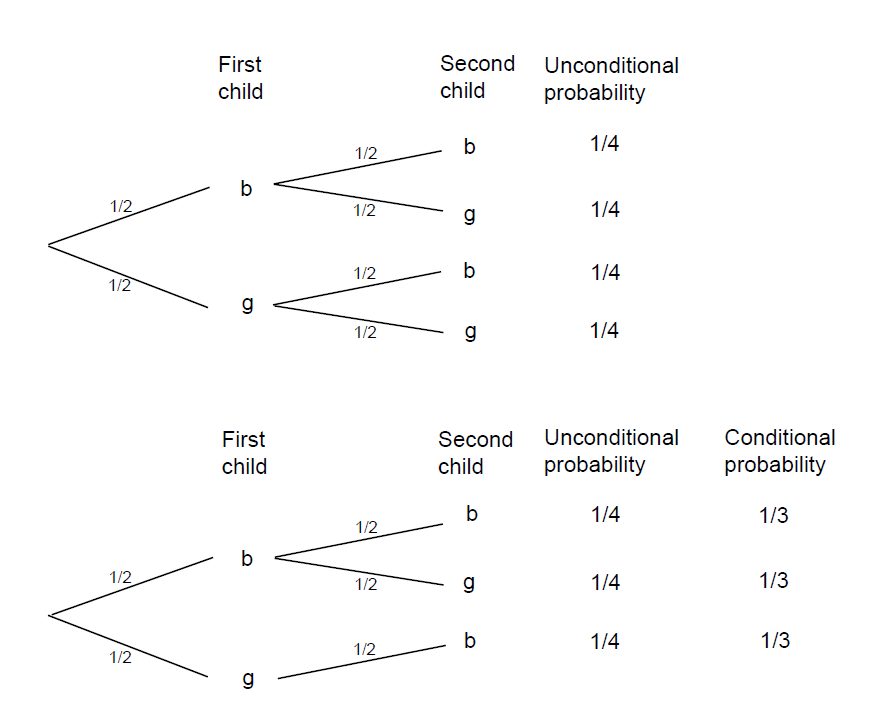
Consider a family with two children. Given that one of the children is a boy, what is the probability that both children are boys?
One way to approach this problem is to say that the other child is equally likely to be a boy or a girl, so the probability that both children are boys is 1/2. The “text-book" solution would be to draw the tree diagram and then form the conditional tree by deleting paths to leave only those paths that are consistent with the given information. The result is shown in Figure \(\PageIndex{1}\). We see that the probability of two boys given a boy in the family is not 1/2 but rather 1/3.
This problem and others like it are discussed in Bar-Hillel and Falk.19 These authors stress that the answer to conditional probabilities of this kind can change depending upon how the information given was actually obtained. For example, they show that 1/2 is the correct answer for the following scenario.
Mr. Smith is the father of two. We meet him walking along the street with a young boy whom he proudly introduces as his son. What is the probability that Mr. Smith’s other child is also a boy?
- Answer
-
As usual we have to make some additional assumptions. For example, we will assume that if Mr. Smith has a boy and a girl, he is equally likely to choose either one to accompany him on his walk. In Figure \(\PageIndex{2}\) we show the tree analysis of this problem and we see that 1/2 is, indeed, the correct answer
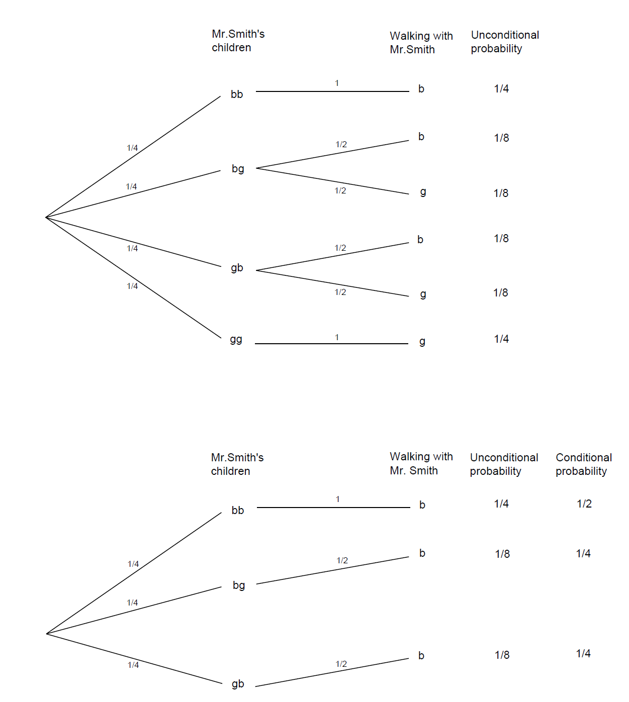
Figure \(\PageIndex{2}\): Tree for example .
It is not so easy to think of reasonable scenarios that would lead to the classical 1/3 answer. An attempt was made by Stephen Geller in proposing this problem to Marilyn vos Savant.20 Geller’s problem is as follows: A shopkeeper says she has two new baby beagles to show you, but she doesn’t know whether they’re both male, both female, or one of each sex. You tell her that you want only a male, and she telephones the fellow who’s giving them a bath. “Is at least one a male?" she asks. “Yes," she informs you with a smile. What is the probability that the other one is male?
The reader is asked to decide whether the model which gives an answer of 1/3 is a reasonable one to use in this case.
In the preceding examples, the apparent paradoxes could easily be resolved by clearly stating the model that is being used and the assumptions that are being made. We now turn to some examples in which the paradoxes are not so easily resolved.
Two envelopes each contain a certain amount of money. One envelope is given to Ali and the other to Baba and they are told that one envelope contains twice as much money as the other. However, neither knows who has the larger prize. Before anyone has opened their envelope, Ali is asked if she would like to trade her envelope with Baba. She reasons as follows: Assume that the amount in my envelope is \(x\). If I switch, I will end up with \(x/2\) with probability 1/2, and \(2x\) with probability 1/2. If I were given the opportunity to play this game many times, and if I were to switch each time, I would, on average, get \[\frac 12 \frac x2 + \frac 12 2x = \frac 54 x\ .\] This is greater than my average winnings if I didn’t switch.
Of course, Baba is presented with the same opportunity and reasons in the same way to conclude that he too would like to switch. So they switch and each thinks that his/her net worth just went up by 25%.
Since neither has yet opened any envelope, this process can be repeated and so again they switch. Now they are back with their original envelopes and yet they think that their fortune has increased 25% twice. By this reasoning, they could convince themselves that by repeatedly switching the envelopes, they could become arbitrarily wealthy. Clearly, something is wrong with the above reasoning, but where is the mistake?
- Answer
-
One of the tricks of making paradoxes is to make them slightly more difficult than is necessary to further befuddle us. As John Finn has suggested, in this paradox we could just have well started with a simpler problem. Suppose Ali and Baba know that I am going to give then either an envelope with $5 or one with $10 and I am going to toss a coin to decide which to give to Ali, and then give the other to Baba. Then Ali can argue that Baba has \(2x\) with probability \(1/2\) and \(x/2\) with probability \(1/2\). This leads Ali to the same conclusion as before. But now it is clear that this is nonsense, since if Ali has the envelope containing $5, Baba cannot possibly have half of this, namely $2.50, since that was not even one of the choices. Similarly, if Ali has $10, Baba cannot have twice as much, namely $20. In fact, in this simpler problem the possibly outcomes are given by the tree diagram in Figure 4.14. From the diagram, it is clear that neither is made better off by switching.
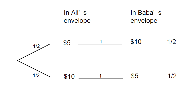
Figure \(\PageIndex{1}\): ohn Finn’s version of Example
In the above example, Ali’s reasoning is incorrect because he infers that if the amount in his envelope is \(x\), then the probability that his envelope contains the smaller amount is 1/2, and the probability that her envelope contains the larger amount is also 1/2. In fact, these conditional probabilities depend upon the distribution of the amounts that are placed in the envelopes.
For definiteness, let \(X\) denote the positive integer-valued random variable which represents the smaller of the two amounts in the envelopes. Suppose, in addition, that we are given the distribution of \(X\), i.e., for each positive integer \(x\), we are given the value of \[p_x = P(X = x)\ .\] (In Finn’s example, \(p_5 = 1\), and \(p_{n} = 0\) for all other values of \(n\).) Then it is easy to calculate the conditional probability that an envelope contains the smaller amount, given that it contains \(x\) dollars. The two possible sample points are \((x, x/2)\) and \((x, 2x)\). If \(x\) is odd, then the first sample point has probability 0, since \(x/2\) is not an integer, so the desired conditional probability is 1 that \(x\) is the smaller amount. If \(x\) is even, then the two sample points have probabilities \(p_{x/2}\) and \(p_x\), respectively, so the conditional probability that \(x\) is the smaller amount is \[\frac{p_x}{p_{x/2} + p_x}\ ,\] which is not necessarily equal to 1/2.
Steven Brams and D. Marc Kilgour21 study the problem, for different distributions, of whether or not one should switch envelopes, if one’s objective is to maximize the long-term average winnings. Let \(x\) be the amount in your envelope. They show that for any distribution of \(X\), there is at least one value of \(x\) such that you should switch. They give an example of a distribution for which there is exactly one value of \(x\) such that you should switch (see Exercise 4.3.5). Perhaps the most interesting case is a distribution in which you should always switch. We now give this example.
Suppose that we have two envelopes in front of us, and that one envelope contains twice the amount of money as the other (both amounts are positive integers). We are given one of the envelopes, and asked if we would like to switch.
- Answer
-
As above, we let \(X\) denote the smaller of the two amounts in the envelopes, and let \[p_x = P(X = x)\ .\] We are now in a position where we can calculate the long-term average winnings, if we switch. (This long-term average is an example of a probabilistic concept known as expectation, and will be discussed in Chapter 6.) Given that one of the two sample points has occurred, the probability that it is the point \((x, x/2)\) is \[\frac{p_{x/2}}{p_{x/2} + p_x}\ ,\] and the probability that it is the point \((x, 2x)\) is \[\frac{p_x}{p_{x/2} + p_x}\ .\] Thus, if we switch, our long-term average winnings are \[\frac{p_{x/2}}{p_{x/2} + p_x}\frac x2 + \frac{p_x}{p_{x/2} + p_x} 2x\ .\] If this is greater than \(x\), then it pays in the long run for us to switch. Some routine algebra shows that the above expression is greater than \(x\) if and only if
\[\frac{p_{x/2}}{p_{x/2} + p_x} < \frac {2}{3}.\]
It is interesting to consider whether there is a distribution on the positive integers such that the inequality is true for all even values of \(x\). Brams and Kilgour22 give the following example.
We define \(p_x\) as follows: \[p_x = \left \{ \matrix{ \frac 13 \Bigl(\frac 23\Bigr)^{k-1}, & \mbox{if}\,\, x = 2^k, \cr 0, & \mbox{otherwise.}\cr }\right.\] It is easy to calculate (see Exercise 4.3.4) that for all relevant values of \(x\), we have \[\frac{p_{x/2}}{p_{x/2} + p_x} = \frac 35\ ,\] which means that the inequality is always true.
So far, we have been able to resolve paradoxes by clearly stating the assumptions being made and by precisely stating the models being used. We end this section by describing a paradox which we cannot resolve.
Suppose that we have two envelopes in front of us, and we are told that the envelopes contain \(X\) and \(Y\) dollars, respectively, where \(X\) and \(Y\) are different positive integers. We randomly choose one of the envelopes, and we open it, revealing \(X\), say. Is it possible to determine, with probability greater than 1/2, whether \(X\) is the smaller of the two dollar amounts?
- Answer
-
Even if we have no knowledge of the joint distribution of \(X\) and \(Y\), the surprising answer is yes! Here’s how to do it. Toss a fair coin until the first time that heads turns up. Let \(Z\) denote the number of tosses required plus 1/2. If \(Z > X\), then we say that \(X\) is the smaller of the two amounts, and if \(Z < X\), then we say that \(X\) is the larger of the two amounts.
First, if \(Z\) lies between \(X\) and \(Y\), then we are sure to be correct. Since \(X\) and \(Y\) are unequal, \(Z\) lies between them with positive probability. Second, if \(Z\) is not between \(X\) and \(Y\), then \(Z\) is either greater than both \(X\) and \(Y\), or is less than both \(X\) and \(Y\). In either case, \(X\) is the smaller of the two amounts with probability 1/2, by symmetry considerations (remember, we chose the envelope at random). Thus, the probability that we are correct is greater than 1/2.
Exercises
Exercise \(\PageIndex{1}\)
One of the first conditional probability paradoxes was provided by Bertrand.23 It is called the Bot Paradox. A cabinet has three drawers. In the first drawer there are two gold balls, in the second drawer there are two silver balls, and in the third drawer there is one silver and one gold ball. A drawer is picked at random and a ball chosen at random from the two balls in the drawer. Given that a gold ball was drawn, what is the probability that the drawer with the two gold balls was chosen?
Exercise \(\PageIndex{2}\)
The following problem is called the two aces problem. This problem, dating back to 1936, has been attributed to the English mathematician J. H. C. Whitehead (see Gridgeman24). This problem was also submitted to Marilyn vos Savant by the master of mathematical puzzles Martin Gardner, who remarks that it is one of his favorites.
A bridge hand has been dealt, i. e. thirteen cards are dealt to each player. Given that your partner has at least one ace, what is the probability that he has at least two aces? Given that your partner has the ace of hearts, what is the probability that he has at least two aces? Answer these questions for a version of bridge in which there are eight cards, namely four aces and four kings, and each player is dealt two cards. (The reader may wish to solve the problem with a 52-card deck.)
Exercise \(\PageIndex{3}\)
In the preceding exercise, it is natural to ask “How do we get the information that the given hand has an ace?" Gridgeman considers two different ways that we might get this information. (Again, assume the deck consists of eight cards.)
- Assume that the person holding the hand is asked to “Name an ace in your hand" and answers “The ace of hearts." What is the probability that he has a second ace?
- Suppose the person holding the hand is asked the more direct question “Do you have the ace of hearts?" and the answer is yes. What is the probability that he has a second ace?
Exercise \(\PageIndex{4}\)
Using the notation introduced in Example 4.3.5, show that in the example of Brams and Kilgour, if \(x\) is a positive power of 2, then \[\frac{p_{x/2}}{p_{x/2} + p_x} = \frac 35\ .\]
Exercise \(\PageIndex{5}\)
Using the notation introduced in Example 4.3.5, let \[p_x = \left \{ \matrix{ \frac 23 \Bigl(\frac 13\Bigr)^k, & \mbox{if}\,\, x = 2^k, \cr 0, & \mbox{otherwise.}\cr }\right.\] Show that there is exactly one value of \(x\) such that if your envelope contains \(x\), then you should switch.
Exercise *\(\PageIndex{6}\)
(For bridge players only. From Sutherland.25) Suppose that we are the declarer in a hand of bridge, and we have the king, 9, 8, 7, and 2 of a certain suit, while the dummy has the ace, 10, 5, and 4 of the same suit. Suppose that we want to play this suit in such a way as to maximize the probability of having no losers in the suit. We begin by leading the 2 to the ace, and we note that the queen drops on our left. We then lead the 10 from the dummy, and our right-hand opponent plays the six (after playing the three on the first round). Should we finesse or play for the drop?