
2.1: Minterms
- Page ID
- 10864

\( \newcommand{\vecs}[1]{\overset { \scriptstyle \rightharpoonup} {\mathbf{#1}} } \)
\( \newcommand{\vecd}[1]{\overset{-\!-\!\rightharpoonup}{\vphantom{a}\smash {#1}}} \)
\( \newcommand{\dsum}{\displaystyle\sum\limits} \)
\( \newcommand{\dint}{\displaystyle\int\limits} \)
\( \newcommand{\dlim}{\displaystyle\lim\limits} \)
\( \newcommand{\id}{\mathrm{id}}\) \( \newcommand{\Span}{\mathrm{span}}\)
( \newcommand{\kernel}{\mathrm{null}\,}\) \( \newcommand{\range}{\mathrm{range}\,}\)
\( \newcommand{\RealPart}{\mathrm{Re}}\) \( \newcommand{\ImaginaryPart}{\mathrm{Im}}\)
\( \newcommand{\Argument}{\mathrm{Arg}}\) \( \newcommand{\norm}[1]{\| #1 \|}\)
\( \newcommand{\inner}[2]{\langle #1, #2 \rangle}\)
\( \newcommand{\Span}{\mathrm{span}}\)
\( \newcommand{\id}{\mathrm{id}}\)
\( \newcommand{\Span}{\mathrm{span}}\)
\( \newcommand{\kernel}{\mathrm{null}\,}\)
\( \newcommand{\range}{\mathrm{range}\,}\)
\( \newcommand{\RealPart}{\mathrm{Re}}\)
\( \newcommand{\ImaginaryPart}{\mathrm{Im}}\)
\( \newcommand{\Argument}{\mathrm{Arg}}\)
\( \newcommand{\norm}[1]{\| #1 \|}\)
\( \newcommand{\inner}[2]{\langle #1, #2 \rangle}\)
\( \newcommand{\Span}{\mathrm{span}}\) \( \newcommand{\AA}{\unicode[.8,0]{x212B}}\)
\( \newcommand{\vectorA}[1]{\vec{#1}} % arrow\)
\( \newcommand{\vectorAt}[1]{\vec{\text{#1}}} % arrow\)
\( \newcommand{\vectorB}[1]{\overset { \scriptstyle \rightharpoonup} {\mathbf{#1}} } \)
\( \newcommand{\vectorC}[1]{\textbf{#1}} \)
\( \newcommand{\vectorD}[1]{\overrightarrow{#1}} \)
\( \newcommand{\vectorDt}[1]{\overrightarrow{\text{#1}}} \)
\( \newcommand{\vectE}[1]{\overset{-\!-\!\rightharpoonup}{\vphantom{a}\smash{\mathbf {#1}}}} \)
\( \newcommand{\vecs}[1]{\overset { \scriptstyle \rightharpoonup} {\mathbf{#1}} } \)
\(\newcommand{\longvect}{\overrightarrow}\)
\( \newcommand{\vecd}[1]{\overset{-\!-\!\rightharpoonup}{\vphantom{a}\smash {#1}}} \)
\(\newcommand{\avec}{\mathbf a}\) \(\newcommand{\bvec}{\mathbf b}\) \(\newcommand{\cvec}{\mathbf c}\) \(\newcommand{\dvec}{\mathbf d}\) \(\newcommand{\dtil}{\widetilde{\mathbf d}}\) \(\newcommand{\evec}{\mathbf e}\) \(\newcommand{\fvec}{\mathbf f}\) \(\newcommand{\nvec}{\mathbf n}\) \(\newcommand{\pvec}{\mathbf p}\) \(\newcommand{\qvec}{\mathbf q}\) \(\newcommand{\svec}{\mathbf s}\) \(\newcommand{\tvec}{\mathbf t}\) \(\newcommand{\uvec}{\mathbf u}\) \(\newcommand{\vvec}{\mathbf v}\) \(\newcommand{\wvec}{\mathbf w}\) \(\newcommand{\xvec}{\mathbf x}\) \(\newcommand{\yvec}{\mathbf y}\) \(\newcommand{\zvec}{\mathbf z}\) \(\newcommand{\rvec}{\mathbf r}\) \(\newcommand{\mvec}{\mathbf m}\) \(\newcommand{\zerovec}{\mathbf 0}\) \(\newcommand{\onevec}{\mathbf 1}\) \(\newcommand{\real}{\mathbb R}\) \(\newcommand{\twovec}[2]{\left[\begin{array}{r}#1 \\ #2 \end{array}\right]}\) \(\newcommand{\ctwovec}[2]{\left[\begin{array}{c}#1 \\ #2 \end{array}\right]}\) \(\newcommand{\threevec}[3]{\left[\begin{array}{r}#1 \\ #2 \\ #3 \end{array}\right]}\) \(\newcommand{\cthreevec}[3]{\left[\begin{array}{c}#1 \\ #2 \\ #3 \end{array}\right]}\) \(\newcommand{\fourvec}[4]{\left[\begin{array}{r}#1 \\ #2 \\ #3 \\ #4 \end{array}\right]}\) \(\newcommand{\cfourvec}[4]{\left[\begin{array}{c}#1 \\ #2 \\ #3 \\ #4 \end{array}\right]}\) \(\newcommand{\fivevec}[5]{\left[\begin{array}{r}#1 \\ #2 \\ #3 \\ #4 \\ #5 \\ \end{array}\right]}\) \(\newcommand{\cfivevec}[5]{\left[\begin{array}{c}#1 \\ #2 \\ #3 \\ #4 \\ #5 \\ \end{array}\right]}\) \(\newcommand{\mattwo}[4]{\left[\begin{array}{rr}#1 \amp #2 \\ #3 \amp #4 \\ \end{array}\right]}\) \(\newcommand{\laspan}[1]{\text{Span}\{#1\}}\) \(\newcommand{\bcal}{\cal B}\) \(\newcommand{\ccal}{\cal C}\) \(\newcommand{\scal}{\cal S}\) \(\newcommand{\wcal}{\cal W}\) \(\newcommand{\ecal}{\cal E}\) \(\newcommand{\coords}[2]{\left\{#1\right\}_{#2}}\) \(\newcommand{\gray}[1]{\color{gray}{#1}}\) \(\newcommand{\lgray}[1]{\color{lightgray}{#1}}\) \(\newcommand{\rank}{\operatorname{rank}}\) \(\newcommand{\row}{\text{Row}}\) \(\newcommand{\col}{\text{Col}}\) \(\renewcommand{\row}{\text{Row}}\) \(\newcommand{\nul}{\text{Nul}}\) \(\newcommand{\var}{\text{Var}}\) \(\newcommand{\corr}{\text{corr}}\) \(\newcommand{\len}[1]{\left|#1\right|}\) \(\newcommand{\bbar}{\overline{\bvec}}\) \(\newcommand{\bhat}{\widehat{\bvec}}\) \(\newcommand{\bperp}{\bvec^\perp}\) \(\newcommand{\xhat}{\widehat{\xvec}}\) \(\newcommand{\vhat}{\widehat{\vvec}}\) \(\newcommand{\uhat}{\widehat{\uvec}}\) \(\newcommand{\what}{\widehat{\wvec}}\) \(\newcommand{\Sighat}{\widehat{\Sigma}}\) \(\newcommand{\lt}{<}\) \(\newcommand{\gt}{>}\) \(\newcommand{\amp}{&}\) \(\definecolor{fillinmathshade}{gray}{0.9}\)Partitions and minterms
To see how the fundamental partition arises naturally, consider first the partition of the basic space produced by a single event \(A\).
\[\Omega = A \bigvee A^c\]
Now if \(B\) is a second event, then
\[A = AB \bigvee AB^c\]
and
\[A^c = A^c B \bigvee A^c B^c\]
so that
\[\Omega = A^c B^c \bigvee A^c B \bigvee AB^c \bigvee AB\]
The pair \(\{A, B\}\) has partitioned \(\Omega\) into \(\{A^c B^c, A^c B, AB^c, AB\}\). Continuation is this way leads systematically to a partition by three events \(\{A, B, C\}\), four events \(\{A, B, C, D\}\), etc.
We illustrate the fundamental patterns in the case of four events \(\{A, B, C, D\}\). We form the minterms as intersections of members of the class, with various patterns of complementation. For a class of four events, there are \(2^4 = 16\) such patterns, hence 16 minterms. These are, in a systematic arrangement,
| \(A^c B^c C^c D^c\) | \(A^c B C^c D^c\) | \(A B^c C^c D^c\) | \(A B C^c D^c\) |
| \(A^c B^c C^c D\) | \(A^c B C^c D\) | \(A B^c C^c D\) | \(A B C^c D\) |
| \(A^c B^c C D^c\) | \(A^c B C D^c\) | \(A B^c C D^c\) | \(A B C D^c\) |
| \(A^c B^c C D\) | \(A^c B C D\) | \(A B^c C D\) | \(A B C D\) |
No element can be in more than one minterm, because each differs from the others by complementation of at least one member event. Each element \(\omega\) is assigned to exactly one of the minterms by determining the answers to four questions:
Is it in \(A\)? Is it in \(B\)? Is it in \(C\)? Is it in \(D\)?
Suppose, for example, the answers are: Yes, No, No, Yes. Then ω is in the minterm \(A B^c C^c D\). In a similar way, we can determine the membership of each \(\omega\) in the basic space. Thus, the minterms form a partition. That is, the minterms represent mutually exclusive events, one of which is sure to occur on each trial. The membership of any minterm depends upon the membership of each generating set \(A, B, C\) or \(D\), and the relationships between them. For some classes, one or more of the minterms are empty (impossible events). As we see below, this causes no problems.
An examination of the development above shows that if we begin with a class of n events, there are \(2^n\) minterms. To aid in systematic handling, we introduce a simple numbering system for the minterms, which we illustrate by considering again the four events \(A, B, C, D\), in that order. The answers to the four questions above can be represented numerically by the scheme
No \(\sim 0\) and Yes \(\sim 1\)
Thus, if \(\omega\) is in \(A^c B^c C^c D^c\), the answers are tabulated as 0 0 0 0. If \(\omega\) is in \(A B^c C^c D\), then this is designated 1 0 0 1. With this scheme, the minterm arrangement above becomes
| 0000 \(\sim\) 0 | 0100 \(\sim\) 4 | 1000 \(\sim\) 8 | 1100 \(\sim\) 12 |
| 0001 \(\sim\) 1 | 0101 \(\sim\) 5 | 1001 \(\sim\) 9 | 1101 \(\sim\) 13 |
| 0010 \(\sim\) 2 | 0110 \(\sim\) 6 | 1010 \(\sim\) 10 | 1110 \(\sim\) 14 |
| 0011 \(\sim\) 3 | 0111 \(\sim\) 7 | 1011 \(\sim\) 11 | 1111 \(\sim\) 15 |
We may view these quadruples of zeros and ones as binary representations of integers, which may also be represented by their decimal equivalents, as shown in the table. Frequently, it is useful to refer to the minterms by number. If the members of the generating class are treated in a fixed order, then each minterm number arrived at in the manner above specifies a minterm uniquely. Thus, for the generating class \(\{A, B, C, D\}\), in that order, we may designate
\(A^c B^c C^c D^c = M_0\) (minterm 0) \(AB^cC^c D = M_9\) (minterm 9), etc.
We utilize this numbering scheme on special Venn diagrams called minterm maps. These are illustrated in Figure, for the cases of three, four, and five generating events. Since the actual content of any minterm depends upon the sets \(A, B, C\), and \(D\) in the generating class, it is customary to refer to these sets as variables. In the three-variable case, set \(A\) is the right half of the diagram and set \(C\) is the lower half; but set B is split, so that it is the union of the second and fourth columns. Similar splits occur in the other cases.
Remark. Other useful arrangements of minterm maps are employed in the analysis of switching circuits.
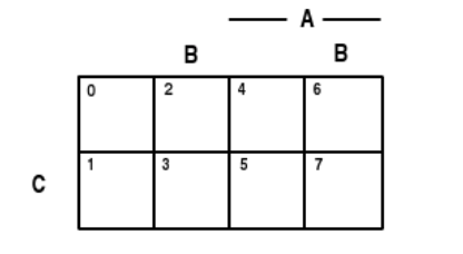
Three variables
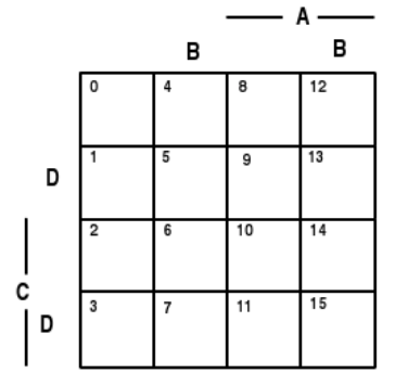
Four variables
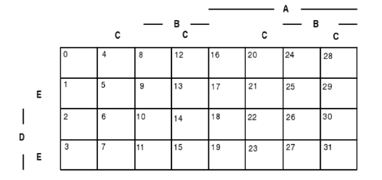
Five variables
Figure 2.1.1. Minterm maps for three, four, or five variables
Minterm maps and the minterm expansion
The significance of the minterm partition of the basic space rests in large measure on the following fact.
Minterm expansion
Each Boolean combination of the elements in a generating class may be expressed as the disjoint union of an appropriate subclass of the minterms. This representation is known as the minterm expansion for the combination.
In deriving an expression for a given Boolean combination which holds for any class \(\{A, B, C, D\}\) of four events, we include all possible minterms, whether empty or not. If a minterm is empty for a given class, its presence does not modify the set content or probability assignment for the Boolean combination.
The existence and uniqueness of the expansion is made plausible by simple examples utilizing minterm maps to determine graphically the minterm content of various Boolean combinations. Using the arrangement and numbering system introduced above, we let \(M_i\) represent the \(i\)th minterm (numbering from zero) and let \(p(i)\) represent the probability of that minterm. When we deal with a union of minterms in a minterm expansion, it is convenient to utilize the shorthand illustrated in the following.
\(M(1, 3, 7) = M_1 \bigvee M_3 \bigvee M_7\) and \(p(1, 3, 7) = p(1) + p(3) + p(7)\)
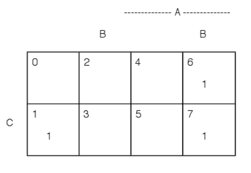
Figure 2.1.2. \(E = AB \cup A^c (B \cup C^c)^c = M(1:6, 7)\) Minterm expansion for Example 2.1.1
Consider the following simple example.
Example \(\PageIndex{1}\) Minterm expansion
Suppose \(E = AB \cup A^c (B \cup C^c)^c\). Examination of the minterm map in Figure 2.1.2 show that \(AB\) consists of the union of minterms \(M_6\), \(M_7\), which we designate \(M(6,7)\). The combination \(B \cup C^c = M(0, 2, 3, 4, 6, 7)\), so that its complement \((B \cup C^c)^c = M(1, 5)\). This leaves the comon part \(A^c (B \cup C^c)^c = M_1\), Hence, \(E = M(1, 6, 7)\). Similarly, \(F = A \cup B^c C = M(1, 4, 5, 6, 7)\).
A key to establishing the expansion is to note that each minterm is either a subset of the combination or is disjoint from it. The expansion is thus the union of those minterms included in the combination. A general verification using indicator functions is sketched in the last section of this module.
Use of minterm maps
A typical problem seeks the probability of certain Boolean combinations of a class of events when the probabilities of various other combinations is given. We consider several simple examples and illustrate the use of minterm maps in formulation and solution.
Example \(\PageIndex{2}\) Survey on software
Statistical data are taken for a certain student population with personal computers. An individual is selected at random. Let \(A =\) the event the person selected has word processing, \(B =\) the event he or she has a spread sheet program, and \(C =\) the event the person has a data base program. The data imply
- The probability is 0.80 that the person has a word processing program: \(P(A) = 0.8\)
- The probability is 0.65 that the person has a spread sheet program: \(P(B) = 0.65\)
- The probability is 0.30 that the person has a data base program: \(P(C) = 0.3\)
- The probability is 0.10 that the person has all three: \(P(ABC) = 0.1\)
- The probability is 0.05 that the person has neither word processing nor spread sheet: \(P(A^c B^c = 0.05\)
- The probability is 0.65 that the person has at least two: \(P(AB \cup AC \cup BC) = 0.65\)
- The probability of word processor and data base, but no spread sheet is twice the probabilty of spread sheet and data base, but no word processor: \(P(AB^cC) = 2P(A^cBC)\)
a. What is the probability that the person has exactly two of the programs?
b. What is the probability that the person has only the data base program?
Several questions arise:
- Are these data consistent?
- Are the data sufficient to answer the questions?
- How may the data be utilized to anwer the questions?
Solution
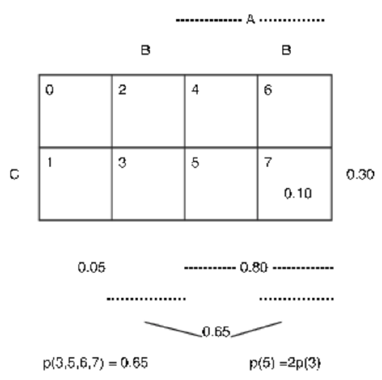
The data, expressed in terms of minterm probabilities, are:
\(P(A) = p(4, 5, 6, 7) = 0.80\); hence \(P(A^c) = p(0, 1, 2, 3) = 0.20\)
\(P(B) = p(2, 3, 6, 7) = 0.65\); hence \(P(B^c) = p(0, 1, 4, 5) = 0.35\)
\(P(C) = p(1, 3, 5, 7) = 0.30\); hence \(P(C^c) = p(0, 2, 4, 6) = 0.70\)
\(P(ABC) = p(7) = 0.10\) \(P(A^c B^c) = p(0, 1) = 0.05\)
\(P(AB \cup AC \cup BC) = p(3, 5, 6, 7) = 0.65\)
\(P(AB^c C) = p(5) = 2p(3) = 2P(A^c BC)\)
These data are shown on the minterm map in Figure 2.1.3 a. We use the patterns displayed in the minterm map to aid in an algebraic solution for the various minterm probabilities.
\(p(2, 3) = p(0, 1, 2, 3) - p(0, 1) = 0.20 - 0.05 = 0.15\)
\(p(6,7) = p(2, 3, 6, 7) - p(2, 3) = 0.65 - 0.15 = 0.50\)
\(p(6) = p(6,7) - p(7) = 0.50 - 0.10 = 0.40\)
\(p(3,5) = p(3, 5, 6, 7) - p(6,7) = 0.65 -0.50 = 0.15 \Rightarrow p(3) = 0.05\),
\(p(5) = 0.10 \Rightarrow p(2) = 0.10\)
\(p(1) = p(1, 3, 5, 7) - p(3, 5) - p(7) = 0.30 - 0.15 - 0.10 = 0.05 \Rightarrow p(0) = 0\)
\(p(4) = p(4, 5, 6, 7) - p(5) - p(6, 7) = 0.80 - 0.10 - 0.50 = 0.20\)
Thus, all minterm probabilities are determined. They are displayed in Figure 2.1.3 b. From these we get
\(P(A^c BC \bigvee AB^cC \bigvee ABC^c) = p(3, 5, 6) = 0.05 + 0.10 + 0.40 = 0.55\) and \(P(A^c B^c C) = p(1) = 0.05\)
a. Data for software survey, Example 2.3.1
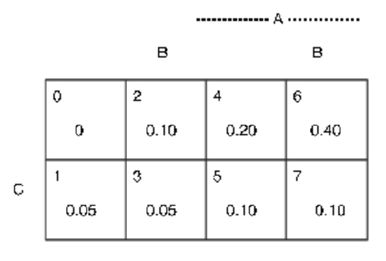
b. Minterm probabilities for software survey. Example 3.3.1
Figure 2.1.3. Minterm maps for software survey.
Example \(\PageIndex{3}\) Survey on personal computers
A survey of 1000 students shows that 565 have PC compatible desktop computers, 515 have Macintosh desktop computers, and 151 have laptop computers. 51 have all three, 124 have both PC and laptop computers, 212 have at least two of the three, and twice as many own both PC and laptop as those who have both Macintosh desktop and laptop. A person is selected at random from this population. What is the probability he or she has at least one of these types of computer? What is the probability the person selected has only a laptop?
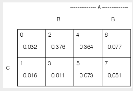
Figure 2.1.4. Minterm probabilities for computer survey. Example 2.1.3
Solution
Let \(A =\) the event of owning a PC desktop, \(B =\) the event of owning a Macintosh desktop, and \(C =\) the event of owning a laptop. We utilize a minterm map for three variables to help determine minterm patterns. For example, the event \(AC = M_5 \bigvee M_7\) so that \(P(AC) = p(5) + p(7) = p(5, 7)\).
The data, expressed in terms of minterm probabilities, are:
\(P(A) = p(4, 5, 6, 7) = 0.565\), hence \(P(A^c) = p(0, 1, 2, 3) = 0.435\)
\(P(B) = p(2, 3, 6, 7) = 0.515\), hence \(P(B^c) = p(0, 1, 4, 5) = 0.485\)
\(P(C) = p(1, 3, 5, 7) = 0.151\), hence \(P(C^c) = p(0, 2, 4, 6) = 0.849\)
\(P(ABC) = p(7) = 0.051\) \(P(AC) = p(5, 7) = 0.124\)
\(P(AB \cup AC \cup BC) = p(3, 5, 6, 7) = 0.212\)
\(P(AC) = p(5, 7) = 2p(3, 7) = 2 P(BC)\)
We use the patterns displayed in the minterm map to aid in an algebraic solution for the various minterm probabilities.
\(p(5) = p(5, 7) - p(7) = 0.124 - 0.051 = 0.073\)
\(p(1, 3) = P(A^c C) = 0.151 - 0.124 = 0.027\) \(P(AC^c) = p(4, 6) = 0.565 - 0.124 = 0.441\)
\(p(3, 7) = P(BC) = 0.124/2 = 0.062\)
\(p(3) = 0.062 - 0.051 = 0.011\)
\(p(6) = p(3, 4, 6, 7) - p(3) - p(5, 7) = 0.212 - 0.011 - 0.124 = 0.077\)
\(p(4) = P(A) - p(6) - p(5, 7) = 0.565 - 0.077 - 0.1124 = 0.364\)
\(p(1) = p(1, 3) - p(3) = 0.027 - 0.11 = 0.016\)
\(p(2) = P(B) - p(3, 7) - p(6) = 0.515 - 0.062 - 0.077 = 0.376\)
\(p(0) = P(C^c) - p(4, 6) - p(2) = 0.849 0.441 - 0.376 = 0.032\)
We have determined the minterm probabilities, which are displayed on the minterm map Figure 2.1.4. We may now compute the probability of any Boolean combination of the generating events \(A, B, C\). Thus,
\(P(A \cup B \cup C) = 1 - P(A^c B^c C^c) - 1 - p(0) = 0.968\) and \(P(A^c B^c C) = p(1) = 0.016\)
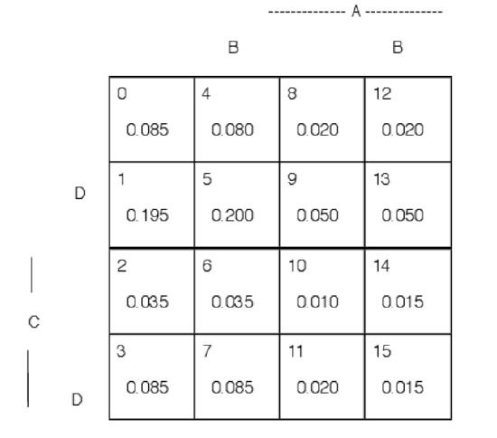
Figure 2.1.5. Minterm probabilities for opinion survey. Example 2.1.4
Example \(\PageIndex{4}\) Opinion survey
A survey of 1000 persons is made to determine their opinions on four propositions. Let \(A, B, C, D\) be the events a person selected agrees with the respective propositions. Survey results show the following probabilities for various combinations:
\(P(A) = 0.200\), \(P(B) = 0.500\), \(P(C) = 0.300\), \(P(D) = 0.700\), \(P(A(B \cup C^c) D^c) = 0.055\)
\(P(A \cup BC \cup D^c) = 0.520\), \(P(A^cBC^c D) = 0.120\), \(P(ABCD) = 0.015\), \(P(AB^c C) = 0.030\)
\(P(A^c B^c C^c D) = 0.195\), \(P(A^c BC) = 0.120\), \(P(A^c B^c D^c) = 0.120\), \(P(AC^c) = 0.140\)
\(P(ACD^c) = 0.025\), \(P(ABC^cD^c) = 0.020\)
Determine the probabilities for each minterm and for each of the following combinations
\(A^c (BC^c \cup B^c C)\) - that is, not \(A\) and (\(B\) or \(C\), but not both)
\(A \cup BC^c\) - that is, \(A\) or (\(B\) and not \(C\))
Solution
At the outset, it is not clear that the data are consistent or sufficient to determine the minterm probabilities. However, an examination of the data shows that there are sixteen items (including the fact that the sum of all minterm probabilities is one). Thus, there is hope, but no assurance, that a solution exists. A step elimination procedure, as in the previous examples, shows that all minterms can in fact be calculated. The results are displayed on the minterm map in Figure 2.1.5. It would be desirable to be able to analyze the problem systematically. The formulation above suggests a more systematic algebraic formulation which should make possible machine aided solution.
Systematic formulation
Use of a minterm map has the advantage of visualizing the minterm expansion in direct relation to the Boolean combination. The algebraic solutions of the previous problems involved ad hoc manipulations of the data minterm probability combinations to find the probability of the desired target combination. We seek a systematic formulation of the data as a set of linear algebraic equations with the minterm probabilities as unknowns, so that standard methods of solution may be employed. Consider again the software survey of Example 2.1.1.
Example \(\PageIndex{5}\) The softerware survey problem reformulated
The data, expressed in terms of minterm probabilities, are:
\(P(A) = p(4, 5, 6, 7) = 0.80\)
\(P(B) = p(2, 3, 6, 7) = 0.65\)
\(P(C) = p(1, 3, 5, 7) = 0.30\)
\(P(ABC) = p(7) = 0.10\)
\(P(A^cB^c) = p(0,1) = 0.05\)
\(P(AB \cup AC \cup BC) = p(3, 5, 6, 7) = 0.65\)
\(P(AB^cC) = p(5) = 2p(3) = 2P(A^cBC)\), so that \(p(5) - 2p(3) = 0\)
We also have in any case
\(P(\Omega) = P(A \cup A^c) = p(0,1, 2, 3, 4, 5, 6, 7) = 1\)
to complete the eight items of data needed for determining all eight minterm probabilities. The first datum can be expressed as an equation in minterm probabilities:
\(0 \cdot p(0) + 0 \cdot p(1) + 0 \cdot p(2) + 0 \cdot p(3) + 1 \cdot p(4) + 1 \cdot p(5) + 1 \cdot p(6) + 1 \cdot p(7) = 0.80\)
This is an algebraic equation in \(p(0), \cdot\cdot\cdot, p(7)\) with a matrix of coefficients
[0 0 0 0 1 1 1 1]
The others may be written out accordingly, giving eight linear algebraic equations in eight variables \(p(0)\) through \(p(7)\). Each equation has a matrix or vector of zero-one coefficients indicating which minterms are included. These may be written in matrix form as follows:
\(\begin{bmatrix} 1 & 1 & 1& & 1 & 1 & 1 & 1 & 1 \\ 0 & 0 & 0 & & 0 & 1 & 1 & 1 & 1 \\ 0 & 0 & 1 & & 1 & 0 & 0 & 1 & 1 \\ 0 & 1 & 0 & & 1 & 0 & 1 & 0 & 1 \\ 0 & 0 & 0 & & 0 & 0 & 0 & 0 & 1 \\ 1 & 1 & 0 & & 0 & 0 & 0 & 0 & 0 \\ 0 & 0 & 0 & & 1 & 0 & 1 & 1 & 1 \\ 0 & 0 & 0 & & -2 & 0 & 1 & 0 & 0 \end{bmatrix} \begin{bmatrix} p(0) \\ p(1) \\ p(2) \\ p(3) \\ p(4) \\ p(5) \\ p(6) \\ p(7) \end{bmatrix} = \begin{bmatrix} 1 \\ 0.80 \\ 0.65 \\ 0.30 \\ 0.10 \\0.05 \\ 0.65 \\ 0 \end{bmatrix} = \begin{bmatrix} P(\Omega) \\ P(A) \\ P(B) \\ P(C) \\ P(ABC) \\ P(A^c B^c) \\ P(AB \cup AC \cup BC) \\ P(AB^cC) - 2P(A^c BC) \end{bmatrix}\)
- The patterns in the coefficient matrix are determined by logical operations. We obtained these with the aid of a minterm map.
- The solution utilizes an algebraic procedure, which could be carried out in a variety of ways, including several standard computer packages for matrix operations.
We show in the module Minterm Vectors and MATLAB how we may use MATLAB for both aspects.
Indicator functions and the minterm expansion
Previous discussion of the indicator function shows that the indicator function for a Boolean combination of sets is a numerical valued function of the indicator functions for the individual sets.
- As an indicator function, it takes on only the values zero and one.
- The value of the indicator function for any Boolean combination must be constant on each minterm. For example, for each ω in the minterm \(AB^cCD^c\), we must have \(I_A(\omega) = 1\), \(I_B(\omega) = 0\), \(I_C(\omega) = 1\), and \(I_D(\omega) = 0\). Thus, any function of \(I_A\), \(I_B\), \(I_C\), \(I_D\) must be constant over the minterm.
- Consider a Boolean combination \(E\) of the generating sets. If \(\omega\) is in \(E \cap M_i\), then \(I_E(\omega) = 1\) for all \(\omega \in M_i\), so that \(M_i \subset E\). Since each \(\omega \in M_i\) or some \(i, E\) must be the union of those minterms sharing an \(\omega\) with \(E\).
- Let \(\{M_i: i \in J_E\}\) be the subclass of those minterms on which \(I_E\) has the value one. Then
\(E = \bigvee_{J_E} M_i\)
which is the minterm expansion of \(E\).