5.2: When Significant Differences are Missed

The problem can run the other way. Scientists routinely judge whether a significant difference exists simply by eye, making use of plots like this one:

Figure \(\PageIndex{1}\)

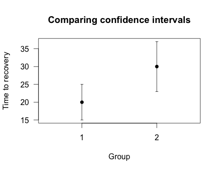
Imagine the two plotted points indicate the estimated time until recovery from some disease in two different groups of patients, each containing ten patients. There are three different things those error bars could represent:

1. The standard deviation of the measurements. Calculate how far each observation is from the average, square each difference, and then average the results and take the square root. This is the standard deviation, and it measures how spread out the measurements are from their mean.
2. The standard error of some estimator. For example, perhaps the error bars are the standard error of the mean. If I were to measure many different samples of patients, each containing exactly \(n\) subjects, I can estimate that \(68\)% of the mean times to recover I measure will be within one standard error of “real” average time to recover. (In the case of estimating means, the standard error is the standard deviation of the measurements divided by the square root of the number of measurements, so the estimate gets better as you get more data – but not too fast.) Many statistical techniques, like least-squares regression, provide standard error estimates for their results.
3. The confidence interval of some estimator. A \(95\)% confidence interval is mathematically constructed to include the true value for \(95\) random samples out of \(100\), so it spans roughly two standard errors in each direction. (In more complicated statistical models this may not be exactly true.)

These three options are all different. The standard deviation is a simple measurement of my data. The standard error tells me how a statistic, like a mean or the slope of a best-fit line, would likely vary if I take many samples of patients. A confidence interval is similar, with an additional guarantee that \(95\)% of \(95\)% confidence intervals should include the “true” value.

In the example plot, we have two \(95\)% confidence intervals which overlap. Many scientists would view this and conclude there is no statistically significant difference between the groups. After all, groups \(1\) and \(2\) might not be different – the average time to recover could be \(25\) in both groups, for example, and the differences only appeared because group \(1\) was lucky this time. But does this mean the difference is not statistically significant? What would the p value be?

In this case, \(p<0.05\). There is a statistically significant difference between the groups, even though the confidence intervals overlap.\(^{[1]}\)

Unfortunately, many scientists skip hypothesis tests and simply glance at plots to see if confidence intervals overlap. This is actually a much more conservative test – requiring confidence intervals to not overlap is akin to requiring \(p<0.01\) in some cases.⁵⁰ It is easy to claim two measurements are not significantly different even when they are.

Conversely, comparing measurements with standard errors or standard deviations will also be misleading, as standard error bars are shorter than confidence interval bars. Two observations might have standard errors which do not overlap, and yet the difference between the two is not statistically significant.

A survey of psychologists, neuroscientists and medical researchers found that the majority made this simple error, with many scientists confusing standard errors, standard deviations, and confidence intervals.⁶ Another survey of climate science papers found that a majority of papers which compared two groups with error bars made the error.³⁷ Even introductory textbooks for experimental scientists, such as An Introduction to Error Analysis, teach students to judge by eye, hardly mentioning formal hypothesis tests at all.

There are, of course, formal statistical procedures which generate confidence intervals which can be compared by eye, and even correct for multiple comparisons automatically. For example, Gabriel comparison intervals are easily interpreted by eye.¹⁹

Overlapping confidence intervals do not mean two values are not significantly different. Similarly, separated standard error bars do not mean two values are significantly different. It’s always best to use the appropriate hypothesis test instead. Your eyeball is not a well-defined statistical procedure.

Footnotes

[1] This was calculated with an unpaired \(t\) test, based on a standard error of \(2.5\) in group \(1\) and \(3.5\) in group \(2\).