Glossary
- Page ID
- 2498
\( \newcommand{\vecs}[1]{\overset { \scriptstyle \rightharpoonup} {\mathbf{#1}} } \)
\( \newcommand{\vecd}[1]{\overset{-\!-\!\rightharpoonup}{\vphantom{a}\smash {#1}}} \)
\( \newcommand{\dsum}{\displaystyle\sum\limits} \)
\( \newcommand{\dint}{\displaystyle\int\limits} \)
\( \newcommand{\dlim}{\displaystyle\lim\limits} \)
\( \newcommand{\id}{\mathrm{id}}\) \( \newcommand{\Span}{\mathrm{span}}\)
( \newcommand{\kernel}{\mathrm{null}\,}\) \( \newcommand{\range}{\mathrm{range}\,}\)
\( \newcommand{\RealPart}{\mathrm{Re}}\) \( \newcommand{\ImaginaryPart}{\mathrm{Im}}\)
\( \newcommand{\Argument}{\mathrm{Arg}}\) \( \newcommand{\norm}[1]{\| #1 \|}\)
\( \newcommand{\inner}[2]{\langle #1, #2 \rangle}\)
\( \newcommand{\Span}{\mathrm{span}}\)
\( \newcommand{\id}{\mathrm{id}}\)
\( \newcommand{\Span}{\mathrm{span}}\)
\( \newcommand{\kernel}{\mathrm{null}\,}\)
\( \newcommand{\range}{\mathrm{range}\,}\)
\( \newcommand{\RealPart}{\mathrm{Re}}\)
\( \newcommand{\ImaginaryPart}{\mathrm{Im}}\)
\( \newcommand{\Argument}{\mathrm{Arg}}\)
\( \newcommand{\norm}[1]{\| #1 \|}\)
\( \newcommand{\inner}[2]{\langle #1, #2 \rangle}\)
\( \newcommand{\Span}{\mathrm{span}}\) \( \newcommand{\AA}{\unicode[.8,0]{x212B}}\)
\( \newcommand{\vectorA}[1]{\vec{#1}} % arrow\)
\( \newcommand{\vectorAt}[1]{\vec{\text{#1}}} % arrow\)
\( \newcommand{\vectorB}[1]{\overset { \scriptstyle \rightharpoonup} {\mathbf{#1}} } \)
\( \newcommand{\vectorC}[1]{\textbf{#1}} \)
\( \newcommand{\vectorD}[1]{\overrightarrow{#1}} \)
\( \newcommand{\vectorDt}[1]{\overrightarrow{\text{#1}}} \)
\( \newcommand{\vectE}[1]{\overset{-\!-\!\rightharpoonup}{\vphantom{a}\smash{\mathbf {#1}}}} \)
\( \newcommand{\vecs}[1]{\overset { \scriptstyle \rightharpoonup} {\mathbf{#1}} } \)
\(\newcommand{\longvect}{\overrightarrow}\)
\( \newcommand{\vecd}[1]{\overset{-\!-\!\rightharpoonup}{\vphantom{a}\smash {#1}}} \)
\(\newcommand{\avec}{\mathbf a}\) \(\newcommand{\bvec}{\mathbf b}\) \(\newcommand{\cvec}{\mathbf c}\) \(\newcommand{\dvec}{\mathbf d}\) \(\newcommand{\dtil}{\widetilde{\mathbf d}}\) \(\newcommand{\evec}{\mathbf e}\) \(\newcommand{\fvec}{\mathbf f}\) \(\newcommand{\nvec}{\mathbf n}\) \(\newcommand{\pvec}{\mathbf p}\) \(\newcommand{\qvec}{\mathbf q}\) \(\newcommand{\svec}{\mathbf s}\) \(\newcommand{\tvec}{\mathbf t}\) \(\newcommand{\uvec}{\mathbf u}\) \(\newcommand{\vvec}{\mathbf v}\) \(\newcommand{\wvec}{\mathbf w}\) \(\newcommand{\xvec}{\mathbf x}\) \(\newcommand{\yvec}{\mathbf y}\) \(\newcommand{\zvec}{\mathbf z}\) \(\newcommand{\rvec}{\mathbf r}\) \(\newcommand{\mvec}{\mathbf m}\) \(\newcommand{\zerovec}{\mathbf 0}\) \(\newcommand{\onevec}{\mathbf 1}\) \(\newcommand{\real}{\mathbb R}\) \(\newcommand{\twovec}[2]{\left[\begin{array}{r}#1 \\ #2 \end{array}\right]}\) \(\newcommand{\ctwovec}[2]{\left[\begin{array}{c}#1 \\ #2 \end{array}\right]}\) \(\newcommand{\threevec}[3]{\left[\begin{array}{r}#1 \\ #2 \\ #3 \end{array}\right]}\) \(\newcommand{\cthreevec}[3]{\left[\begin{array}{c}#1 \\ #2 \\ #3 \end{array}\right]}\) \(\newcommand{\fourvec}[4]{\left[\begin{array}{r}#1 \\ #2 \\ #3 \\ #4 \end{array}\right]}\) \(\newcommand{\cfourvec}[4]{\left[\begin{array}{c}#1 \\ #2 \\ #3 \\ #4 \end{array}\right]}\) \(\newcommand{\fivevec}[5]{\left[\begin{array}{r}#1 \\ #2 \\ #3 \\ #4 \\ #5 \\ \end{array}\right]}\) \(\newcommand{\cfivevec}[5]{\left[\begin{array}{c}#1 \\ #2 \\ #3 \\ #4 \\ #5 \\ \end{array}\right]}\) \(\newcommand{\mattwo}[4]{\left[\begin{array}{rr}#1 \amp #2 \\ #3 \amp #4 \\ \end{array}\right]}\) \(\newcommand{\laspan}[1]{\text{Span}\{#1\}}\) \(\newcommand{\bcal}{\cal B}\) \(\newcommand{\ccal}{\cal C}\) \(\newcommand{\scal}{\cal S}\) \(\newcommand{\wcal}{\cal W}\) \(\newcommand{\ecal}{\cal E}\) \(\newcommand{\coords}[2]{\left\{#1\right\}_{#2}}\) \(\newcommand{\gray}[1]{\color{gray}{#1}}\) \(\newcommand{\lgray}[1]{\color{lightgray}{#1}}\) \(\newcommand{\rank}{\operatorname{rank}}\) \(\newcommand{\row}{\text{Row}}\) \(\newcommand{\col}{\text{Col}}\) \(\renewcommand{\row}{\text{Row}}\) \(\newcommand{\nul}{\text{Nul}}\) \(\newcommand{\var}{\text{Var}}\) \(\newcommand{\corr}{\text{corr}}\) \(\newcommand{\len}[1]{\left|#1\right|}\) \(\newcommand{\bbar}{\overline{\bvec}}\) \(\newcommand{\bhat}{\widehat{\bvec}}\) \(\newcommand{\bperp}{\bvec^\perp}\) \(\newcommand{\xhat}{\widehat{\xvec}}\) \(\newcommand{\vhat}{\widehat{\vvec}}\) \(\newcommand{\uhat}{\widehat{\uvec}}\) \(\newcommand{\what}{\widehat{\wvec}}\) \(\newcommand{\Sighat}{\widehat{\Sigma}}\) \(\newcommand{\lt}{<}\) \(\newcommand{\gt}{>}\) \(\newcommand{\amp}{&}\) \(\definecolor{fillinmathshade}{gray}{0.9}\)Learning Objectives
- Definitions of various terms occurring throughout the textbook
A Priori Comparison / Planned Comparison
A comparison that is planned before conducting the experiment or at least before the data are examined. Also called an a priori comparison.
Absolute Deviation / Absolute Difference
The absolute value of the difference between two numbers. The absolute deviation between \(5\) and \(3\) is \(2\); between \(3\) and \(5\) is \(2\); and between \(-4\) and \(2\) it is \(6\).
Alternative Hypothesis
In hypothesis testing, the null hypothesis and an alternative hypothesis are put forward. If the data are sufficiently strong to reject the null hypothesis, then the null hypothesis is rejected in favor of an alternative hypothesis. For instance, if the null hypothesis were that \(μ_1= μ_2\) then the alternative hypothesis (for a two-tailed test) would be \(μ_1 ≠ μ_2\) .
Analysis of Variance
Analysis of variance is a method for testing hypotheses about means. It is the most widely-used method of statistical inference for the analysis of experimental data.
Anti-log
Taking the anti-log of a number undoes the operation of taking the log. Therefore, since \(\log_{10}(1000)= 3\), the \(antilog_{10}\) of \(3\) is \(1,000\).Taking the anti-log of a number undoes the operation of taking the log. Therefore, since \(\log_{10}(1000)= 3\), the \(antilog_{10}\) of \(3\) is \(1,000\). Taking the antilog of \(X\) raises the base of the logarithm in question to \(X\).
Average
- The (arithmetic) mean
- Any measure of central tendency
Bar Chart
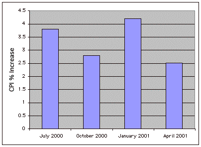
A graphical method of presenting data. A bar is drawn for each level of a variable. The height of each bar contains the value of the variable. Bar charts are useful for displaying things such as frequency counts and percent increases. They are not recommended for displaying means (despite the widespread practice) since box plots present more information in the same amount of space.
An example bar chart is shown below.
Base Rate
The true proportion of a population having some condition, attribute or disease. For example, the proportion of people with schizophrenia is about \(0.01\). It is very important to consider the base rate when classifying people. As the saying goes, "if you hear hoofs, think horse not zebra" since you are more likely to encounter a horse than a zebra (at least in most places.)
Bayes' Theorem
Bayes' theorem considers both the prior probability of an event and the diagnostic value of a test to determine the posterior probability of the event. The theorem is shown below:
\[P(D\mid T) = \frac{P(T\mid D)P(D)}{P(T\mid D)P(D)+P(T\mid D')P(D')}\]
where \(P(D|T)\) is the posterior probability of condition \(D\) given test result \(T\), \(P(T|D)\) is the conditional probability of \(T\) given \(D\), \(P(D)\) is the prior probability of \(D\), \(P(T|D')\) is the conditional probability of \(T\) given not \(D\), and \(P(D')\) is the probability of not \(D'\).
Beta-carotene
The human body converts beta-carotene into Vitamin \(A\), an essential component of our diets. Many vegetables, such as carrots, are good sources of beta-carotene. Studies have suggested beta-carotene supplements may provide a range of health benefits, ranging from promoting healthy eyes to preventing cancer. Other studies have found that beta-carotene supplements may increase the incidence of cancer.
Beta weight
A standardized regression coefficient.
Between-Subjects Factor / Between-Subjects Variable
Between-subject variables are independent variables or factors in which a different group of subjects is used for each level of the variable. If an experiment is conducted comparing four methods of teaching vocabulary and if a different group of subjects is used for each of the four teaching methods, then teaching method is a between-subjects variable.
Bias
- A sampling method is biased if each element does not have an equal chance of being selected. A sample of internet users found reading an online statistics book would be a biased sample of all internet users. A random sample is unbiased. Note that possible bias refers to the sampling method, not the result. An unbiased method could, by chance, lead to a very non-representative sample.
- An estimator is biased if it systematically overestimates or underestimates the parameter it is estimating. In other words, it is biased if the mean of the sampling distribution of the statistic is not the parameter it is estimating, The sample mean is an unbiased estimate of the population mean. The mean squared deviation of sample scores from their mean is a biased estimate of the variance since it tends to underestimate the population variance.
Bimodal Distribution
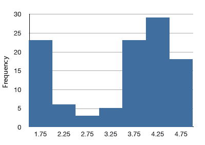
A distribution with two distinct peaks. An example is shown below.
Binomial Distribution
A probability distribution for independent events for which there are only two possible outcomes such as a coin flip. If one of the two outcomes is defined as a success, then the probability of exactly x successes out of \(N\) trials (events) is given by:
\[P(x) = \frac{N!}{x!(N-x)!}\pi ^x(1-\pi )^{N-x}\]
Bivariate
Bivariate data is data for which there are two variables for each observation. As an example, the following bivariate data show the ages of husbands and wives of \(10\) married couples.
| Husband | 36 | 72 | 37 | 36 | 51 | 50 | 47 | 50 | 37 | 41 |
| Wife | 35 | 67 | 33 | 35 | 50 | 46 | 47 | 42 | 36 | 41 |
Bonferroni correction
In general, to keep the familywise error rate (\(FER\)) at or below \(0.05\), the per-comparison error rate (\(PCER\)) should be: \[PCER = 0.05/c\] where \(c\) is the number of comparisons. More generally, to insure that the \(FER\) is less than or equal to alpha, use \[PCER = alpha/c\]
Box Plot
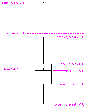
One of the more effective graphical summaries of a data set, the box plot generally shows mean, median, \(25^{th}\) and \(75^{th}\) percentiles, and outliers. A standard box plot is composed of the median, upper hinge, lower hinge, upper adjacent value, lower adjacent value, outside values, and far out values. An example is shown below. Parallel box plots are very useful for comparing distributions. See also: step, H-spread.
Center (of a distribution) / Central Tendency
The center or middle of a distribution. There are many measures of central tendency. The most common are the mean, median, and, mode. Others include the trimean, trimmed mean, and geometric mean.)
Class Frequency
One of the components of a histogram, the class frequency is the number of observations in each class interval.
Class Interval / Bin Width
Also known as bin width, the class interval is a division of data for use in a histogram. For instance, it is possible to partition scores on a \(100\) point test into class intervals of \(1-25\), \(26-49\), \(50-74\) and \(75-100\).
Comparison Among Means/ Contrast Among Means
A method for testing differences among means for significance. For example, one might test whether the difference between \(\text{Mean 1}\) and the average of \(\text{Mean 2}\) and \(\text{Mean 3}\) is significantly different.
Conditional Probability
The probability that \(\text{event A}\) occurs given that \(\text{event B}\) has already occurred is called the conditional probability of \(A\) given \(B\). Symbolically, this is written as \(P(A|B)\). The probability it rains on Monday given that it rained on Sunday would be written as \(\text{P(Rain on Monday | Rain on Sunday)}\).
Confidence Interval
A confidence interval is a range of scores likely to contain the parameter being estimated. Intervals can be constructed to be more or less likely to contain the parameter: \(95\%\) of \(95\%\) confidence intervals contain the estimated parameter whereas \(99\%\) of \(99\%\) confidence intervals contain the estimated parameter. The wider the confidence interval, the more uncertainty there is about the value of the parameter.
Confounding
Two or more variables are confounded if their effects cannot be separated because they vary together. For example, if a study on the effect of light inadvertently manipulated heat along with light, then light and heat would be confounded.
Cook's D
Cook's D is a measure of the influence of an observation in regression and is proportional to the sum of the squared differences between predictions made with all observations in the analysis and predictions made leaving out the observation in question.
Constant
A value that does not change. Values such as pi, or the mass of the Earth are constants. Compare with variables.
Continuous Variables
Variables that can take on any value in a certain range. Time and distance are continuous; gender, SAT score and “time rounded to the nearest second” are not. Variables that are not continuous are known as discrete variables. No measured variable is truly continuous; however, discrete variables measured with enough precision can often be considered continuous for practical purposes.
Correlated Pairs t test / Related Pairs t test
A test of the difference between means of two conditions when there are pairs of scores. Typically, each pair of scores is from a different subject.
Counterbalanced
Counterbalancing is a method of avoiding confounding among variables. Consider an experiment in which subjects are tested on both an auditory reaction time task (in which subjects respond to an auditory stimulus) and a visual reaction time task (in which subjects respond to a visual stimulus). Half of the subjects are given the visual task first and the other half of the subjects are given the auditory task first. That way, there is no confounding of order of presentation and task.
Consumer Price Index - CPI
Also known as the cost of living index, the CPI is a financial statistic that measures the change in price of a representative group of goods over time.
Criterion Variable
In regression analysis (such as linear regression) the criterion variable is the variable being predicted. In general, the criterion variable is the dependent variable.
Cumulative Frequency Distribution
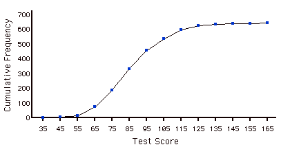
A distribution showing the number of observations less than or equal to values on the \(X\)-axis. The following graph shows a cumulative distribution for scores on a test.
Cumulative Frequency Polygon
A frequency polygon whose vertices represent the sum of all previous class frequencies of the data. For example, if a frequency polygon had vertices of \(5, 8, 3, 7, 10\), the cumulative frequency polygon on the same data would have vertices of \(5, 13, 16, 23, 33\). As another example, a cumulative frequency distribution for scores on a psychology test is shown below.

Data
A collection of values to be used for statistical analysis.
Dependent Variable
A variable that measures the experimental outcome. In most experiments, the effects of the independent variable on the dependent variables are observed. For example, if a study investigated the effectiveness of an experimental treatment for depression, then the measure of depression would be the dependent variable.
Synonym: dependent measure
Descriptive Statistics
- The branch of statistics concerned with describing and summarizing data.
- A set of statistics such as the mean, standard deviation, and skew that describe a distribution.
Deviation Scores
Scores that are expressed as differences (deviations) from some value, usually the mean. To convert data to deviation scores typically means to subtract the mean score from each other score. Thus, the values \(1\), \(2\), and \(3\) in deviation-score form would be computed by subtracting the mean of \(2\) from each value and would be \(-1, 0, 1\).
Degrees of Freedom - df
The degrees of freedom of an estimate is the number of independent pieces of information that go into the estimate. In general, the degrees of freedom for an estimate is equal to the number of values minus the number of parameters estimated en route to the estimate in question. For example, to estimate the population variance, one must first estimate the population mean. Therefore, if the estimate of variance is based on \(N\) observations, there are \(N - 1\) degrees of freedom.
Discrete Variable
Variables that can only take on a finite number of values are called "discrete variables." All qualitative variables are discrete. Some quantitative variables are discrete, such as performance rated as \(1\),\(2\),\(3\),\(4\), or \(5\), or temperature rounded to the nearest degree. Sometimes, a variable that takes on enough discrete values can be considered to be continuous for practical purposes. One example is time to the nearest millisecond.
Variables that can take on an infinite number of possible values are called "continuous variables."
Distribution / Frequency Distribution
The distribution of empirical data is called a frequency distribution and consists of a count of the number of occurrences of each value. If the data are continuous, then a grouped frequency distribution is used. Typically, a distribution is portrayed using a frequency polygon or a histogram.
Mathematical equations are often used to define distributions. The normal distribution is, perhaps, the best known example. Many empirical distributions are approximated well by mathematical distributions such as the normal distribution.
Expected Value
The expected value of a statistic is the mean of the sampling distribution of the statistic. It can be loosely thought of as the long-run average value of the statistic.
Factor / Independent Variables
Variables that are manipulated by the experimenter, as opposed to dependent variables. Most experiments consist of observing the effect of the independent variable(s) on the dependent variable(s).
Factorial Design
In a factorial design, each level of each independent variable is paired with each level of each other independent variable. Thus, a \(2 \times 3\) factorial design consists of the \(6\) possible combinations of the levels of the independent variables.
False Positive
A false positive occurs when a diagnostic procedure returns a positive result while the true state of the subject is negative. For example, if a test for strep says the patient has strep when in fact he or she does not, then the error in diagnosis would be called a false positive. In some contexts, a false positive is called a false alarm. The concept is similar to a Type I error in significance testing.
Familywise Error Rate
When a series of significance tests is conducted, the familywise error rate (\(FER\)) is the probability that one or more of the significance tests results in a Type I error.
Far Out Value
One of the components of a box plot, far out values are those that are more than \(2\) steps from the nearest hinge. They are beyond the outer fences.
Favorable Outcome
A favorable outcome is the outcome of interest. For example one could define a favorable outcome in the flip of a coin as a head. The term "favorable outcome" does not necessarily mean that the outcome is desirable – in some experiments, the favorable outcome could be the failure of a test, or the occurrence of an undesirable event.
Frequency Distribution
For a discrete variable, a frequency distribution consists of the distribution of the number of occurrences for each value of the variable. For a continuous variable, it is the number of occurrences for a variety of ranges of variables.
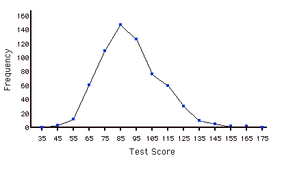
Frequency Polygon
A frequency polygon is a graphical representation of a distribution. It partitions the variable on the \(x\)-axis into various contiguous class intervals of (usually) equal widths. The heights of the polygon's points represent the class frequencies.
Frequency Table
A table containing the number of occurrences in each class of data; for example, the number of each color of M&Ms in a bag. Frequency tables often used to create histograms and frequency polygons. When a frequency table is created for a quantitative variable, a grouped frequency table is generally used.
Grouped Frequency Table
A grouped frequency table shows the number of values for various ranges of scores. Below is shown a grouped frequency table for response times (in milliseconds) for a simple motor task.
| Range | Frequency |
| 500-600 | 3 |
| 600-700 | 6 |
| 700-800 | 5 |
| 800-900 | 5 |
| 900-1000 | 0 |
| 1000-1100 | 1 |
Geometric Mean
The geometric mean is a measure of central tendency. The geometric mean of n numbers is obtained by multiplying all of them together, and then taking the \(n^{th}\) root of them. For example, for the numbers \(1\), \(10\), and \(100\), the product of all the numbers is: \(1 \times 10 \times 100 = 1,000\). Since there are three numbers, we take the cubed root of the product (\(1,000\)) which is equal to \(10\).
Graphs / Graphics
Graphs are often the most effective way to describe distributions and relationships among variables. Among the most common graphs are histograms, box plots, bar charts, and scatterplots.
Grouped Frequency Distribution
A grouped frequency distribution is a frequency distribution in which frequencies are displayed for ranges of data rather than for individual values. For example, the distribution of heights might be calculated by defining one-inch ranges. The frequency of individuals with various heights rounded off to the nearest inch would then be tabulated.
Harmonic Mean
The harmonic mean of n numbers (\(X_1\) to \(X_n\)) is computed using the following formula:
\[\mathit{Harmonic\; Mean} = \frac{n}{\tfrac{1}{x_1}+\tfrac{1}{x_2}+\cdots +\tfrac{1}{x_n}}\]
Often the harmonic mean of sample sizes is computed.
Histogram
A histogram is a graphical representation of a distribution . It partitions the variable on the \(x\)-axis into various contiguous class intervals of (usually) equal widths. The heights of the bars represent the class frequencies.

History Effect
A problem of confounding where the passage of time, and not the variable of interest, is responsible for observed effects.
Homogeneity of variance
The assumption that the variances of all the populations are equal.
Homoscedasticity
In linear regression, the assumption that the variance around the regression line is the same for all values of the predictor variable.
H-spread
One of the components of a box plot, the \(H\)-spread is the difference between the upper hinge and the lower hinge.
iMac
A line of computers released by Apple in \(1998\), that tried to make computers both more accessible (greater ease of use) and fashionable (they came in a line of designer colors.)
Independence
Two variables are said to be independent if the value of one variable provides no information about the value of the other variable. These two variables would be uncorrelated so that Pearson's r would be \(0\).
Two events are independent if the probability the second event occurring is the same regardless of whether or not the first event occurred.
Independent Events
Events \(A\) and \(B\) are independent events if the probability of Event \(B\) occurring is the same whether or not Event \(A\) occurs. For example, if you throw two dice, the probability that the second die comes up \(1\) is independent of whether the first die came up \(1\). Formally, this can be stated in terms of conditional probabilities:
\[P(A|B) = P(A)\\ P(B|A) = P(B)\]
Inference
The act of drawing conclusions about a population from a sample.
Inferential Statistics
The branch of statistics concerned with drawing conclusions about a population from a sample. This is generally done through random sampling, followed by inferences made about central tendency, or any of a number of other aspects of a distribution.
Influence
Influence refers to the degree to which a single observation in regression influences the estimation of the regression parameters. It is often measured in terms how much the predicted scores for other observations would differ if the observation in question were not included.
Inner Fence
In a box plot, the lower inner fence is one step below the lower hinge while the upper inner fence is one step above the upper hinge.
Interaction
Two independent variables interact if the effect of one of the variables differs depending on the level of the other variable.
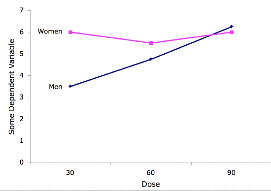
Interaction Plot
An interaction plot displays the levels of one variable on the \(X\) axis and has a separate line for the means of each level of the other variable. The \(Y\) axis is the dependent variable. A look at this graph shows that the effect of dosage is different for males than it is for females.
Interquartile Range
The Interquartile Range (\(IQR\)) is the (\(75^{th}\) percentile – \(25^{th}\) percentile). It is a robust measure of variability.
Interval Estimate
An interval estimate is a range of scores likely to contain the estimated parameter.
Interval Scales
One of \(4\) Levels of Measurement, interval scales are numerical scales in which intervals have the same interpretation throughout. As an example, consider the Fahrenheit scale of temperature. The difference between \(30\) degrees and \(40\) degrees represents the same temperature difference as the difference between \(80\) degrees and \(90\) degrees. This is because each \(10\) degree interval has the same physical meaning (in terms of the kinetic energy. Unlike ratio scales, interval scales do not have a true zero point.
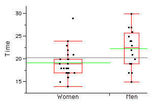
Jitter
When points in a graph are jittered, the are moved horizontally so that all the points can be seen and none are hidden due to overlapping values. An example is shown below:
Kurtosis
Kurtosis measures how fat or thin the tails of a distribution are relative to a normal distribution. It is commonly defined as:
\[\sum \frac{(X-\mu )^4}{\sigma ^4} - 3\]
Distributions with long tails are called leptokurtic; distributions with short tails are called platykurtic. Normal distributions have zero kurtosis.
Leptokurtic
A distribution with long tails relative to a normal distribution is leptokurtic.
Level / Level of a variable / Level of a factor
When a factor consists of various treatment conditions, each treatment condition is considered a level of that factor. For example, if the factor were drug dosage, and three doses were tested, then each dosage would be one level of the factor and the factor would have three levels.
Levels of Measurement
Measurement scales differ in their level of measurement. There are four common levels of measurement:
- Nominal scales are only labels.
- Ordinal Scales are ordered but are not truly quantitative. Equal intervals on the ordinal scale do not imply equal intervals on the underlying trait.
- Interval scales are are ordered and equal intervals equal intervals on the underlying trait. However, interval scales do not have a true zero point.
- Ratio scales are interval scales that do have a true zero point. With ratio scales, it is sensible to talk about one value being twice as large as another, for example.
Leverage
Leverage is a factor affecting the influence of an observation in regression. Leverage is based on how much the observation's value on the predictor variable differs from the mean of the predictor variable. The greater an observation's leverage, the more potential it has to be an influential observation.
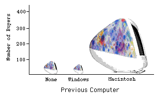
Lie Factor
Many problems can arise when fancy graphs are used over plain ones. Distortions can occur when the heights of objects are used to indicate the value because most people will pay attention to the areas of the objects rather than their height. The lie factor is the ratio of the effect apparent in the graph to actual effect in the data; if it deviates by more than \(0.05\) from \(1\), the graph is generally unacceptable. The lie factor in the following graph is almost \(6\).
Lies
There are three types of lies:
- regular lies
- damned lies
- statistics
This is according to Benjamin Disraeli as quoted by Mark Twain.
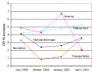
Line Graph
Essentially a bar graph in which the height of each par is represented by a single point, with each of these points connected by a line. Line graphs are best used to show change over time, and should never be used if your \(X\)-axis is not an ordered variable. An example is shown below.
Linear Combination
A linear combination of variables is a way of creating a new variable by combining other variables. A linear combination is one in which each variable is multiplied by a coefficient and the are products summed. For example, if
\[Y = 3X_1 + 2X_2 + 0.5X_3\]
then \(Y\) is a linear combination of the variables \(X_1\), \(X_2\), and \(X_3\).
Linear Regression
Linear regression is a method for predicting a criterion variable from one or more predictor variable. In simple regression, the criterion is predicted from a single predictor variable and the best-fitting straight line is of the form:
\[Y' = bX + A\]
where \(Y'\) is the predicted score, \(X\) is the predictor variable, \(b\) is the slope, and \(A\) is the \(Y\) intercept. Typically, the criterion for the "best fitting" line is the line for which the sum of the squared errors of prediction is minimized. In multiple regression, the criterion is predicted from two or more predictor variables.
Linear Relationship
There is a perfect linear relationship between two variables if a scatterplot of the points falls on a straight line. The relationship is linear even if the points diverge from the line as long as the divergence is random rather than being systematic.
Linear Transformation
A linear transformation is any transformation of a variable that can be achieved by multiplying it by a constant, and then adding a second constant. If \(Y\) is the transformed value of \(X\), then \(Y = aX + b\). The transformation from degrees Fahrenheit to degrees Centigrade is linear and is done using the formula:
\[C = 0.55556F - 17.7778\]
Logarithm - Log
The logarithm of a number is the power the base of the logarithm has to be raised to in order to equal the number. If the base of the logarithm is \(10\) and the number is \(1,000\) then the log is \(3\) since \(10\) has to be raised to the \(3^{rd}\) power to equal \(1,000\).
Lower Adjacent Value
A component of a box plot, the lower adjacent value is smallest value in the data above the inner lower fence.
Lower Hinge
A component of a box plot, the lower hinge is the \(25^{th}\) percentile. The upper hinge is the \(75^{th}\) percentile.
M & M’s
A type of candy consisting of chocolate inside a shell. M & M's come in a variety of colors.
Main Effect
A main effect of an independent variable is the effect of the variable averaging over all levels of the other variable(s). For example, in a design with age and gender as factors, the main effect of gender would be the difference between the genders averaging across all ages used in the experiment.
Margin of Error
When a statistic is used to estimate a parameter, it is common to compute a confidence interval. The margin of error is the difference between the statistic and the endpoints of the interval. For example, if the statistic were \(0.6\) and the confidence interval ranged from \(0.4\) to \(0.8\), then the margin of error would be \(0.20\). Unless otherwise specified, the \(95\%\) confidence interval is used.
Marginal Mean
In a design with two factors, the marginal means for one factor are the means for that factor averaged across all levels of the other factor. In the table shown below, the two factors are "Relationship" and "Companion Weight." The marginal means for each of the two levels of Relationship (Girl Friend and Acquaintance) are computed by averaging across the two levels of Companion Weight. Thus, the marginal mean for Acquaintance of \(6.37\) is the mean of \(6.15\) and \(6.59\).
|
Companion Weight
|
||||
|
|
Obese
|
Typical
|
Marginal Mean
|
|
| Relationship |
Girl Friend
|
5.65
|
6.19
|
5.92
|
|
Acquaintance
|
6.15
|
6.59
|
6.37
|
|
|
Marginal Mean
|
5.90
|
6.39
|
||
Mean / Arithmetic Mean
Also known as the arithmetic mean, the mean is typically what is meant by the word “average.” The mean is perhaps the most common measure of central tendency. The mean of a variable is given by (the sum of all its values)/(the number of values). For example, the mean of \(4\), \(8\), and \(9\) is \(7\). The sample mean is written as M, and the population mean as the Greek letter mu (\(μ\)). Despite its popularity, the mean may not be an appropriate measure of central tendency for skewed distributions, or in situations with outliers.
Median
The median is a popular measure of central tendency. It is the \(50^{th}\) percentile of a distribution. To find the median of a number of values, first order them, then find the observation in the middle: the median of \(5, 2, 7, 9, 4\) is \(5\). (Note that if there is an even number of values, one takes the average of the middle two: the median of \(4, 6, 8,10\) is \(7\).) The median is often more appropriate than the mean in skewed distributions and in situations with outliers.
Miss
Misses occur when a diagnostic test returns a negative result, but the true state of the subject is positive. For example, if a person has strep throat and the diagnostic test fails to indicate it, then a miss has occurred. The concept is similar to a Type II error in significance testing.
Mode
The mode is a measure of central tendency. It is the most frequent value in a distribution: the mode of \(3, 4, 4, 5, 5, 5, 8\) is \(5\). Note that the mode may be very different from the mean and the median.
Multiple Regression
Multiple regression is linear regression in which two or more predictor variables are used to predict the criterion.
Negative Association
There is a negative association between variables \(X\) and \(Y\) if smaller values of \(X\) are associated with larger values of \(Y\) and larger values of \(X\) are associated with smaller values of \(Y\).
Nominal Scale
A nominal scale is one of four commonly-used Levels of Measurement. No ordering is implied, and addition/subtraction and multiplication/division would be inappropriate for a variable on a nominal scale. {Female, Male} and {Buddhist, Christian, Hindu, Muslim} have no natural ordering (except alphabetic). Occasionally, numeric values are nominal: for instance, if a variable were coded as \(\text{Female = 1, Male = 2}\), the set \({1,2}\) is still nominal.
Non representative
A non-representative sample is a sample that does not accurately reflect the population.
Normal Distribution
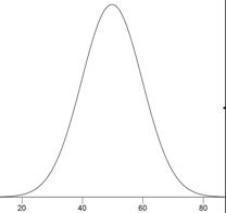
One of the most common continuous distributions, a normal distribution is sometimes referred to as a "bell-shaped distribution." If \(μ\) is the distribution mean, and \(σ\) the standard deviation, then the height (ordinate) normal distribution is given by
\[\frac{1}{\sqrt{2\pi \sigma ^2}}e^{\tfrac{-(x-\mu )^2}{2\sigma ^2}}\]
A graph of a normal distribution with a mean of \(50\) and a standard deviation of \(10\) is shown below.
If the mean is \(0\) and the standard deviation is \(1\), the distribution is referred to as the "standard normal distribution."
Null Hypothesis
A null hypothesis is a hypothesis tested in significance testing. It is typically the hypothesis that a parameter is zero or that a difference between parameters is zero. For example, the null hypothesis might be that the difference between population means is zero. Experimenters typically design experiments to allow the null hypothesis to be rejected.
Omninus Null Hypothesis
The null hypothesis that all population means are equal.
One-Tailed Test / One-Tailed Probability / Directional Test
The last step in significance testing involves calculating the probability that a statistic would differ as much or more from the parameter specified in the null hypothesis as does the statistics obtained in the experiment.
A probability computed considering differences in only one direction, such as the statistic is larger than the parameter, is called a one-tailed probability. For example, if a parameter is \(0\) and the statistic is \(12\), a one-tailed probability (the positive tail) would be the probability of a statistic being \(≥12\). Compare with the two-tailed probability which would be the probability of being either \(≤ -12\) or \(≥12\).
Ordinal Scale
One of four commonly used levels of measurement, an ordinal scale is a set of ordered values. However, there is no set distance between scale values. For instance, for the scale: (Very Poor, Poor, Average, Good, Very Good) is an ordinal scale. You can assign numerical values to an ordinal scale: rating performance such as \(1\) for "Very Poor," \(2\) for "Poor," etc, but there is no assurance that the difference between a score of \(1\) and \(2\) means the same thing as the difference between a score of \(2\) and \(3\).
Orthogonal Comparisons
When comparisons among means provide completely independent information, the comparisons are called "orthogonal." If an experiment with four groups were conducted, then a comparison of \(\text{Groups 1 and 2}\) would be orthogonal to a comparison of \(\text{Groups 3 and 4}\) since there is nothing in the comparison of \(\text{Groups 1 and 2}\) that provides information about the comparison of \(\text{Groups 3 and 4}\).
Outer Fence
In a box plot, the lower outer fence is \(2\) steps below the lower hinge whereas the upper inner fence is \(2\) steps above the upper hinge.
Outlier
Outliers are atypical, infrequent observations; values that have an extreme deviation from the center of the distribution. There is no universally-agreed on criterion for defining an outlier, and outliers should only be discarded with extreme caution. However, one should always assess the effects of outliers on the statistical conclusions.
Outside Value
A component of a box plot, outside values are more than \(1\) step beyond the nearest hinge. They are beyond an inner fence but not beyond an outer fence.
Pairwise Comparisons
Pairwise comparisons are comparisons between pairs of means.
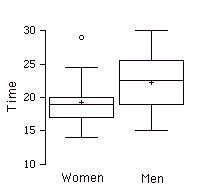
Parallel Box Plots
Two or more box plots drawn on the same \(Y\)-axis. These are often useful in comparing features of distributions. An example portraying the times it took samples of women and men to do a task is shown below.
Parameter
A value calculated in a population. For example, the mean of the numbers in a population is a parameter. Compare with a statistic, which is a value computed in a sample to estimate a parameter.
Partial Slope
The partial slope in multiple regression is the slope of the relationship between a predictor variable that is independent of the other predictor variables and the criterion. It is also the regression coefficient for the predictor variable in question.
Pearson's \(r\) / Pearson's Product Moment Correlation / Pearson's Correlation
Pearson's correlation is a measure of the strength of the linear relationship between two variables. It ranges from \(-1\) for a perfect negative relationship to \(+1\) for a perfect positive relationship. A correlation of \(0\) means that there is no linear relationship.
Percentile
There is no universally accepted definition of a percentile. Using the \(65^{th}\) percentile as an example, some statisticians define the \(65^{th}\) percentile as the lowest score that is greater than \(65\%\) of the scores. Others have defined the \(65^{th}\) percentile as the lowest score that is greater than or equal to \(65\%\) of the scores. A more sophisticated definition is given below. The first step is to compute the rank (\(R\)) of the percentile in question. This is done using the following formula:
\[R = \frac{P}{100} \times (N + 1)\]
where \(P\) is the desired percentile and \(N\) is the number of numbers. If \(R\) is an integer, then the \(P^{th}\) percentile is the number with rank \(R\). When \(R\) is not an integer, we compute the \(P^{th}\) percentile by interpolation as follows:
- Define \(IR\) as the integer portion of \(R\) (the number to the left of the decimal point).
- Define \(FR\) as the fractional portion or \(R\).
- Find the scores with Rank \(IR\) and with Rank \(IR + 1\).
- Interpolate by multiplying the difference between the scores by \(FR\) and add the result to the lower score.
Per-Comparison Error Rate
The per-comparison error rate refers to the Type I error rate of any one significance test conducted as part of a series of significance tests. Thus, if \(10\) significance tests were each conducted at \(0.05\) significance level, then the per-comparison error rate would be \(0.05\). Compare with the familywise error rate.
Pie Chart
A graphical representation of data, the pie chart shows relative frequencies of classes of data. It is a circle cut into a number of wedges, one for each class, with the area of each wedge proportional to its relative frequency. Pie charts are only effective for a small number of classes, and are one of the less effective graphical representations.
Placebo
A device used in clinical trials, the placebo is visually indistinguishable from the study medication, but in reality has no medical effect (often, a sugar pill). A group of subjects chosen randomly takes the placebo, the others take one or another type of medication. This is done to prevent confounding the medical and psychological effects of the drug. Even a sugar pill can lead some patients to report improvement and side effects.
Planned Comparison / A Priori Comparison
A comparison that is planned before conducting the experiment or at least before the data are examined. Also called an a priori comparison.
Platykurtic
A distribution with short tails relative to a normal distribution is platykurtic.
Point Estimate
When a parameter is being estimated, the estimate can be either a single number or it can be a range of numbers such as in a confidence interval. When the estimate is a single number, the estimate is called a "point estimate."
Polynomial Regression
Polynomial regression is a form of multiple regression in which powers of a predictor variable instead of other predictor variables are used. In the following example, the criterion (\(Y\)) is predicted by \(X\), \(X^2\) and, \(X^3\).
\[Y = b_1X + b_2X^2 + b_3X^3 + A\]
Population
A population is the complete set of observations a researcher is interested in. Contrast this with a sample which is a subset of a population. A population can be defined in a manner convenient for a researcher. For example, one could define a population as all girls in fourth grade in Houston, Texas. Or, a different population is the set of all girls in fourth grade in the United States. Inferential statistics are computed from sample data in order to make inferences about the population.
Positive Association
There is a positive association between variables \(X\) and \(Y\) if smaller values of \(X\) are associated with smaller values of \(Y\) and larger values of \(X\) are associated with larger values of \(Y\).
Posterior Probability
The posterior probability of an event is the probability of the event computed following the collection of new data. One begins with a prior probability of an event and revises it in the light of new data. For example, if \(0.01\) of a population has schizophrenia then the probability that a person drawn at random would have schizophrenia is \(0.01\). This is the prior probability. If you then learn that that their score on a personality test suggests the person is schizophrenic, you would adjust your probability accordingly. The adjusted probability is the posterior probability.
Power
In significance testing, power is the probability of rejecting a false null hypothesis.
Precision
A statistic's precision concerns to how close it is expected to be to the parameter it is estimating. Precise statistics are vary less from sample to sample. The precision of a statistic is usually defined in terms of it standard error.
Predictor Variable
A predictor variable is a variable used in regression to predict another variable. It is sometimes referred to as an independent variable if it is manipulated rather than just measured.
Prior Probability
The prior probability of an event is the probability of the event computed before the collection of new data. One begins with a prior probability of an event and revises it in the light of new data. For example, if \(0.01\) of a population has schizophrenia then the probability that a person drawn at random would have schizophrenia is \(0.01\). This is the prior probability. If you then learn that that there score on a personality test suggests the person is schizophrenic, you would adjust your probability accordingly. The adjusted probability is the posterior probability.
Probability Density Function
For a discrete random variable, a probability distribution contains the probability of each possible outcome. However, for a continuous random variable, the probability of any one outcome is zero (if you specify it to enough decimal places). A probability density function is a formula that can be used to compute probabilities of a range of outcomes for a continuous random variable. The sum of all densities is always \(1.0\) and the value of the function is always greater or equal to zero.
Probability Distribution
For a discrete random variable, a probability distribution contains the probability of each possible outcome. The sum of all probabilities is always \(1.0\).
Probability Value / \(p\) value
In significance testing, the probability value (sometimes called the \(p\) value) is the probability of obtaining a statistic as different or more different from the parameter specified in the null hypothesis as the statistic obtained in the experiment. The probability value is computed assuming the null hypothesis is true. The lower the probability value, the stronger the evidence that the null hypothesis is false. Traditionally, the null hypothesis is rejected if the probability value is below \(0.05\).
Probability values can be either one tailed or two tailed.
Qualitative Variables / Categorical Variable
Also known as categorical variables, qualitative variables are variables with no natural sense of ordering. They are therefore measured on a nominal scale. For instance, hair color (Black, Brown, Gray, Red, Yellow) is a qualitative variable, as is name (Adam, Becky, Christina, Dave . . .). Qualitative variables can be coded to appear numeric but their numbers are meaningless, as in \(\text{male=1, female=2}\). Variables that are not qualitative are known as quantitative variables.
Quantitative Variable
Variables that are measured on a numeric or quantitative scale. Ordinal, interval and ratio scales are quantitative. A country’s population, a person’s shoe size, or a car’s speed are all quantitative variables. Variables that are not quantitative are known as qualitative variables.
Random Assignment
Random assignment occurs when the subjects in an experiment are randomly assigned to conditions. Random assignment prevents systematic confounding of treatment effects with other variables.
Random Sampling / Simple Random Sampling
The process of selecting a subset of a population for the purposes of statistical inference. Random sampling means that every member of the population is equally likely to be chosen.
Range
The difference between the maximum and minimum values of a variable or distribution. The range is the simplest measure of variability.
Ratio Scale
One of the four basic levels of measurement, a ratio scale is a numerical scale with a true zero point and in which a given size interval has the same interpretation for the entire scale. Weight is a ratio scale, Therefore, it is meaningful to say that a \(200\) pound person weighs twice as much as a \(100\) pound person.
Regression
Regression means "prediction." The regression of \(Y\) on \(X\) means the prediction of \(Y\) by \(X\).
Regression Coefficient
A regression coefficient is the slope of the regression line in simple regression or the partial slope in multiple regression.
Regression Line
In linear regression, the line of best fit is called the regression line.
Relative frequency
The proportion of observations falling into a given class. For example, if a bag of \(55\) M & M's has \(11\) green M&M's, then the frequency of green M&M's is \(11\) and the relative frequency is \(11/55 = 0.20\). Relative frequencies are often used in histograms, pie charts, and bar graphs.
Relative Frequency Distribution
A relative frequency distribution is just like a frequency distribution except that it consists of the proportions of occurrences instead of the numbers of occurrences for each value (or range of values) of a variable.
Reliability
Although there are many ways to conceive of the reliability of a test, the classical way is to define the reliability as the correlation between two parallel forms of the test. When defined this way, the reliability is the ratio of true score variance to test score variance. Chronbach's \(α\) is a common measure of reliability.
Repeated-Measures Factor / Repeated-Measures Variable / Within-Subjects Factor /Within-Subjects Variable
A within-subjects variable is an independent variable that is manipulated by testing each subject at each level of the variable. Compare with a between-subjects variable in which different groups of subjects are used for each level of the variable.
Representative Sample
A representative sample is a sample chosen to match the qualities of the population from which it is drawn. With a large sample size, random sampling will approximate a representative sample; stratified random sampling can be used to make a small sample more representative.
Robust
Something is robust if it holds up well in the face of adversity. A measure of central tendency or variability is considered robust if it is not greatly affected by a few extreme scores. A statistical test is considered robust if it works well in spite of moderate violations of the assumptions on which it is based.
Sample
A sample is a subset of a population, often taken for the purpose of statistical inference. Generally, one uses a random sample.
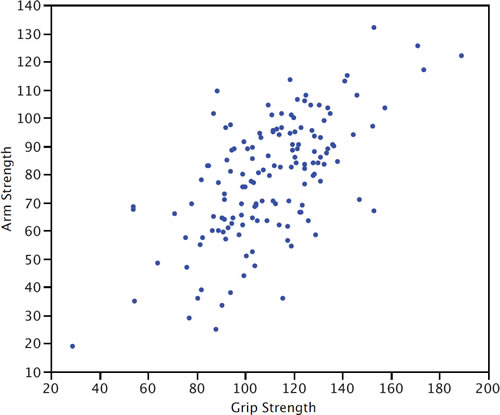
Scatter Plot
A scatter plot of two variables shows the values of one variable on the \(Y\) axis and the values of the other variable on the \(X\) axis. Scatter plots are well suited for revealing the relationship between two variables. The scatter plot shown below illustrates the relationship between grip strength and arm strength in a sample of workers.
Semi-Interquartile Range
The semi interquartile range is the interquartile range divided by \(2\). It is a robust measure of variability. The Interquartile Range is the (\(75^{th}\) percentile \(–\) \(25^{th}\) percentile).
Significance Level / A level
In significance testing, the significance level is the highest value of a probability value for which the null hypothesis is rejected. Common significance levels are \(0.05\) and \(0.01\). If the \(0.05\) level is used, then the null hypothesis is rejected if the probability value is less than or equal to \(0.05\).
Significance Testing / Hypothesis Testing / Significant Difference
A statistical procedure that tests the viability of the null hypothesis. If data (or more extreme data) are very unlikely given that the null hypothesis is true, then the null hypothesis is rejected. If the data or more extreme data are not unlikely, then the null hypothesis is not rejected. If the null hypothesis is rejected, then the result of the test is said to be significant. A statistically significant effect does not mean the effect is important.
Simple Effect
The simple effect of a factor is the effect of that factor at a single level of another factor. For example, in a design with age and gender as factors, the effect of age for females would be one of the simple effects of age.
Simple Regression
Simple regression is linear regression in which one more predictor variable is used to predict the criterion.
Skew
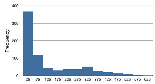
A distribution is skewed if one tail extends out further than the other. A distribution has positive skew (is skewed to the right) if the tail to the right is longer. See the graph below for an example.
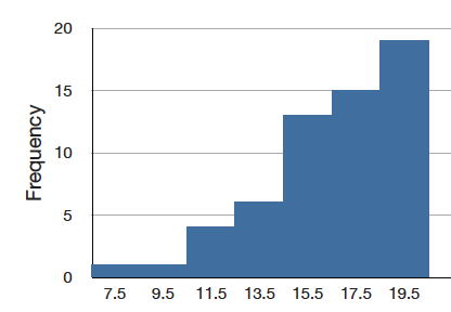
A distribution has a negative skew (is skewed to the left) if the tail to the left is longer. See the graph below for an example.
Slope
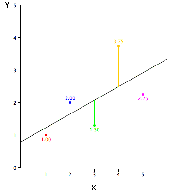
The slope of a line is the change in \(Y\) for each change of one unit of \(X\). It is sometimes defined as "rise over run" which is the same thing. The slope of the black line in the graph is \(0.425\) because the line increases by \(0.425\) each time \(X\) increases by \(1.0\).
Squared Deviation
A squared deviation is the difference between two values, squared. The number that minimizes the sum of squared deviations for a variable is its mean.
Standard Deviation
The standard deviation is a widely used measure of variability. It is computed by taking the square root of the variance. An important attribute of the standard deviation as a measure of variability is that if the mean and standard deviation of a normal distribution are known, it is possible to compute the percentile rank associated with any given score.
Standard Error
The standard error of a statistic is the standard deviation of the sampling distribution of that statistic. For example, the standard error of the mean is the standard deviation of the sampling distribution of the mean. Standard errors play a critical role in constructing confidence intervals and in significance testing.
Standard Error of Measurement
In test theory, the standard error of measurement is the standard deviation of observed test scores for a given true score. It is usually estimated with the following formula in which \(s\) is the standard deviation of the test scores and \(r\) is the reliability of the test.
\[S_{measurement} = s\sqrt{1-r}\]
Standard Error of the Mean
The standard error of the mean is the standard deviation of the sampling distribution of the mean. The formula for the standard error of the mean in a population is:
\[\sigma _m = \frac{\sigma }{\sqrt{N}}\]
where \(σ\) is the standard deviation and \(N\) is the sample size. When computed in a sample, the estimate of the standard error of the mean is:
\[s_m = \frac{s}{\sqrt{N}}\]
Standard Normal Distribution
The standard normal distribution is a normal distribution with a mean of \(0\) and a standard deviation of \(1\).
Standard Score / Standardize / Standard Normal Deviate / \(Z\) score
The number of standard deviations a score is from the mean of its population. The term "standard score" is usually used for normal populations; the terms "\(Z\) score" and "normal deviate" should only be used in reference to normal distributions. The transformation from a raw score \(X\) to a \(Z\) score can be done using the following formula:
\[Z = \frac{X - \mu}{\sigma }\]
Transforming a variable in this way is called "standardizing" the variable. It should be kept in mind that if \(X\) is not normally distributed then the transformed variable will not be normally distributed either.
Standardize / Standard Score
A variable is standardized if it has a mean of \(0\) and a standard deviation of \(1\). The transformation from a raw score \(X\) to a standard score can be done using the following formula:
\[X_{standardized} = \frac{X - \mu}{\sigma }\]
where \(μ\) is the mean and \(σ\) is the standard deviation. Transforming a variable in this way is called "standardizing" the variable. It should be kept in mind that if \(X\) is not normally distributed then the transformed variable will not be normally distributed either.
Statistics / Statistic
- What you are studying right now, also known as statistical analysis, or statistical inference. It is a field of study concerned with summarizing data, interpreting data, and making decisions based on data.
- A quantity calculated in a sample to estimate a value in a population is called a "statistic."
Stem and Leaf Display
A quasi-graphical representation of numerical data. Generally, all but the final digit of each value is a stem, the final digit is the leaf. The stems are placed in a vertical list, with each matched leaf on one side. They can be very useful for visualizing small data sets with no more than two significant digits. An example is shown below. In this example, you multiply the stems by \(10\) and add the value of the leaf to obtain the numeric value. Thus the maximum number of touchdown passes is \(3 \times 10 + 7 = 37\).
Stem and leaf display of the number of touchdown passes:
\[\begin{array}{c|c c c c c c c c c c c c c c c } 3 & 2 & 3 & 3 & 7 \\ 2 &0 &0 &1 &1 &1 &2 &2 &2 &3 &8 &8 &9\\ 1 &2 &2 &4 &4 &4 &5 &6 &8 &8 &8 &8 &9 &9\\ 0 &6 &9 \end{array}\]
Step
One of the components of a box plot, the step is \(1.5\) times the difference between the upper hinge and the lower hinge.
Stratified Random Sampling
In stratified random sampling, the population is divided into a number of subgroups (or strata). Random samples are then taken from each subgroup with sample sizes proportional to the size of the subgroup in the population. For instance, if a population contained equal numbers of men and women, and the variable of interest is suspected to vary by gender, one might conduct stratified random sampling to insure a representative sample.
Studentized Range Distribution
The studentized range distribution is used to test the difference between the largest and smallest means. It is similar to the \(t\) distribution which is used when there are only two means.
Sturgis’ Rule
One method of determining the number of classes for a histogram, Sturgis’ Rule is to take \(1 + \log _2(N)\) classes, rounded to the nearest integer.
Sum of Squares Error
In linear regression, the sum of squares error is the sum of squared errors of prediction. In analysis of variance, it is the sum of squared deviations from cell means for between-subjects factors and the \(\text{Subjects x Treatment}\) interaction for within-subject factors.
Symmetric Distribution
In a symmetric distribution, the upper and lower halves of the distribution are mirror images of each other. For example, in the distribution shown below, the portions above and below \(50\) are mirror images of each other. In a symmetric distribution, the mean is equal to the median. Antonym: skewed distribution.

\(t\) distribution
The \(t\) distribution is the distribution of a value sampled from a normal distribution divided by an estimate of the distribution's standard deviation. In practice the value is typically a statistic such as the mean or the difference between means and the standard deviation is an estimate of the standard error of the statistic. The \(t\) distribution in leptokurtic.
\(t\) test
Most commonly, a significance test of the difference between means based on the t distribution. Other applications include
- testing the significance of the difference between a sample mean and a hypothesized value of the mean and
- testing a specific contrast among means
Third Variable Problem
A type of confounding in which a third variable leads to a mistaken causal relationship between two others. For instance, cities with a greater number of churches have a higher crime rate. However, more churches do not lead to more crime, but instead the third variable, population, leads to both more churches and more crime.
Touchdown Pass
In American football, a touchdown pass occurs when a completed pass results in a touchdown. The pass may be to a player in the end zone or to a player who subsequently runs into the end zone. A touchdown is worth \(6\) points and allows for a chance at one (and by some rules two) additional point(s).
Trimean
The trimean is a robust measure of central tendency; it is a weighted average of the \(25^{th}\), \(50^{th}\), and \(75^{th}\) percentiles. Specifically it is computed as follows:
\[\mathrm{Trimean} = 0.25 \times 25^{th} + 0.5 \times 50^{th} + 0.25 \times 75^{th}\]
True Score
In classical test theory, the true score is a theoretical value that represents a test taker's score without error. If a person took parallel forms of a test thousands of times (assuming no practice or fatigue effects), the mean of all their scores would be a good approximation of their true score since the error would be almost entirely averaged out. It should be distinguished from validity.
Tukey HSD Test
The "Honestly Significantly Different" (\(HSD\)) test developed by the statistician John Tukey to test all pairwise comparisons among means. The test is based on the "studentized range distribution."
Two-Tailed Test / Two-Tailed Probability / Non-directional Test
The last step in significance testing involves calculating the probability that a statistic would differ as much or more from the parameter specified in the null hypothesis as does the statistics obtained in the experiment.
A probability computed considering differences in both direction (statistic either larger or smaller than the parameter) is called two-tailed probability. For example, if a parameter is \(0\) and the statistic is \(12\), a two-tailed probability would be the he probability of being either \(≤ -12\) or \(≥12\). Compare with the one-tailed probability which would be the probability of a statistic being \(≥\) to \(12\) if that were the direction specified in advance.
Type I error
In significance testing, the error of rejecting a true null hypothesis.
Type II error
In significance testing, the failure to reject a false null hypothesis.
Unbiased
A sample is said to be unbiased when every individual has an equal chance of being chosen from the population.
An estimator is unbiased if it does not systematically overestimate or underestimate the parameter it is estimating. In other words, it is unbiased if the mean of the sampling distribution of the statistic is the parameter it is estimating, The sample mean is an unbiased estimate of the population mean.
Unplanned Comparisons / Post Hoc Comparisons
When the comparison among means is decided on after viewing the data, the comparison is called an "unplanned comparison" or a post-hoc comparison. Different statistical tests are required for unplanned comparisons than for planned comparisons.
Upper Adjacent Value
One of the components of a box plot, the higher adjacent value is the largest value in the data below the \(75^{th}\) percentile.
Upper hinge
The upper hinge is one of the components of a box plot; it is the \(75^{th}\) percentile.
Variability / Spread
Variability refers to the extent to which values differ from one another. That is, how much they vary. Variability can also be thought of as how spread out a distribution is. The standard deviation and the semi-interquartile range are measures of variability.
Variable
Something that can take on different values. For example, different subjects in an experiment weigh different amounts. Therefore "weight" is a variable in the experiment. Or, subjects may be given different doses of a drug. This would make "dosage" a variable. Variables can be dependent or independent, qualitative or quantitative, and continuous or discrete.
Variance
The variance is a widely used measure of variability. It is defined as the mean squared deviation of scores from the mean. The formula for variance computed in an entire population is
\[\sigma ^2 = \frac{\sum (X-\mu )^2}{N}\]
where \(σ^2\) represents the variance, \(μ\) is the mean, and \(N\) is the number of scores.
When computed in a sample in order to estimate the variance in the population, the population is
\[s^2 = \frac{\sum (X-M)^2}{N-1}\]
where \(s^2\) is the estimate of variance, \(M\) is the sample mean, and \(N\) is the number of scores in the sample.
Variance Sum Law
The variance sum law is an expression for the variance of the sum of two variables. If the variables are independent and therefore Pearson's \(r = 0\), the following formula represents the variance of the sum and difference of the variables \(X\) and \(Y\):
\[\sigma _{X\pm Y}^{2} = \sigma _{X}^{2} + \sigma _{Y}^{2}\]
Note that you add the variances for both \(X + Y\) and \(X - Y\).
If \(X\) and \(Y\) are correlated, then the following formula (which the former is a special case) should be used:
\[\sigma _{X\pm Y}^{2} = \sigma _{X}^{2} + \sigma _{Y}^{2} \pm 2\rho \sigma _X \sigma _Y\]
where \(ρ\) is the population value of the correlation. In a sample \(r\) is used as an estimate of \(ρ\).
Within-Subjects Design
An experimental design in which the independent variable is a within-subjects variable.
Within-Subjects Factor / Within-Subjects Variable / Repeated-Measures Factor / Repeated-Measures Variable
A within-subjects variable is an independent variable that is manipulated by testing each subject at each level of the variable. Compare with a between-subjects variable in which different groups of subjects are used for each level of the variable.
Y-Intercept
The \(Y\)-intercept of a line is the value of \(Y\) at the point that the line intercepts the \(Y\) axis. It is the value of \(Y\) when \(X\) equals \(0\). The \(Y\) intercept of the black line shown in the graph is \(0.785\).

\(Z\) score / Standard Score / Standardize /Standard Normal Deviate
The number of standard deviations a score is from the mean of its population. The term "standard score" is usually used for normal populations; the terms "\(Z\) score" and "normal deviate" should only be used in reference to normal distributions. The transformation from a raw score \(X\) to a \(Z\) score can be done using the following formula:
\[Z = \frac{X-\mu }{\sigma }\]
Transforming a variable in this way is called "standardizing" the variable. It should be kept in mind that if \(X\) is not normally distributed then the transformed variable will not be normally distributed either.


