
2.2: Measures of Central Location - Three Kinds of Averages
- Page ID
- 556
- To learn the concept of the “center” of a data set.
- To learn the meaning of each of three measures of the center of a data set—the mean, the median, and the mode—and how to compute each one.
This section is be titled “three kinds of averages” because any kind of average could be used to answer the question "where is the center of the data?". We will see that the nature of the data set, as indicated by a relative frequency histogram, will determine what constitutes a good answer. Different shapes of the histogram call for different measures of central location.
The Mean
The first measure of central location is the usual “average” that is familiar to everyone: add up all the values, then divide by the number of values. Before writing a formula for the mean let us introduce some handy mathematical notation.
The Greek letter \(\sum \), pronounced "sigma", is a handy mathematical shorthand that stands for "add up all the values" or "sum". For example \(\sum x\) means "add up all the values of \(x\)", and \(\sum x^2\) means "add up all the values of \(x^2\)". In these expressions \(x\) usually stands for a value of the data, so \(\sum x\) stands for "the sum of all the data values" and \(\sum x^2\) means "the sum of the squares of all the data values".
\(\mathbf{n}\) stands for the sample size, the number of data values. An example will help make this clear.
Find \(n\), \(\sum x\), \(\sum x^2\) and \(\sum (x - 1)^2\) for the data:
\[1,\, 3,\, 4 \nonumber \]
Solution
\[\begin{array}{rcl} n & = & 3 \quad \mbox{ because there are three data values} \\ \sum x & = & 1 + 3 + 4 = 8 \\ \sum x^2 & = & 1^2 + 3^2 + 4^2 = 1 + 9 + 16 = 26 \\ \sum {(x - 1)}^2 & = & {(1 - 1)}^2 + {(3 - 1)}^2 + {(4 - 1)}^2 = 0^2 + 2^2 + 3^2 = 13\end{array} \nonumber \]
Using these handy notations it's easy to write a formula defining the mean \(\bar{x}\) of a sample.
The sample mean of a set of \(n\) sample data values is the number \(\bar x\) defined by the formula
\[\bar x = \dfrac{\sum x}{n} \label{samplemean} \]
Find the mean of the following sample data: \(2\), \(-1\), \(0\), \(2\)
Solution
This is a application of Equation \ref{samplemean}:
\[\bar x = \dfrac{\sum x}{n} = \dfrac{2 + (-1) + 0 + 2}{4} = \dfrac{3}{4} = 0.75 \nonumber \]
A random sample of ten students is taken from the student body of a college and their GPAs are recorded as follows:
\[1.90, 3.00, 2.53, 3.71, 2.12, 1.76, 2.71, 1.39, 4.00, 3.33\nonumber \]
Find the mean.
Solution
This is a application of Equation \ref{samplemean}:
\[\begin{array}{rcl}\bar x = \dfrac{\sum x}{n} = \dfrac{1.90 + 3.00 + 2.53 + 3.71 + 2.12 + 1.76 + 2.71 + 1.39 + 4.00 + 3.33}{10} = \dfrac{26.45}{10} = 2.645\end{array} \nonumber \]
A random sample of \(19\) women beyond child-bearing age gave the following data, where \(x\) is the number of children and \(f\) is the frequency, or the number of times it occurred in the data set.
\[\begin{array}{c|cccc}x & 0 & 1 & 2 & 3 & 4 \\ \hline f & 3 & 6 & 6 & 3 & 1\end{array} \nonumber \]
Find the sample mean.
Solution
In this example the data are presented by means of a data frequency table, introduced in Chapter 1. Each number in the first line of the table is a number that appears in the data set; the number below it is how many times it occurs. Thus the value \(0\) is observed three times, that is, three of the measurements in the data set are \(0\), the value \(1\) is observed six times, and so on. In the context of the problem this means that three women in the sample have had no children, six have had exactly one child, and so on. The explicit list of all the observations in this data set is therefore:
\[0, 0, 0, 1, 1, 1, 1, 1, 1, 2, 2, 2, 2, 2, 2, 3, 3, 3, 4 \nonumber \]
The sample size can be read directly from the table, without first listing the entire data set, as the sum of the frequencies: \(n = 3 + 6 + 6 + 3 + 1 = 19\). The sample mean can be computed directly from the table as well:
\[\bar x = \dfrac{\sum x}{n} = \dfrac{0 \times 3 + 1 \times 6 + 2 \times 6 + 3 \times 3 + 4 \times 1}{19} = \dfrac{31}{19} = 1.6316 \nonumber \]
In the examples above the data sets were described as samples. Therefore the means were sample means \(\bar x\). If the data come from a census, so that there is a measurement for every element of the population, then the mean is calculated by exactly the same process of summing all the measurements and dividing by how many of them there are, but it is now the population mean and is denoted by \(\mu\), the lower case Greek letter mu.
The population mean of a set of \(N\) population data is the number \(\mu\) defined by the formula:
\[\displaystyle \mu=\frac{\sum x}{N}. \nonumber \]
The mean of two numbers is the number that is halfway between them. For example, the average of the numbers \(5\) and \(17\) is \((5 + 17) ∕ 2 = 11\), which is \(6\) units above \(5\) and \(6\) units below \(17\). In this sense the average \(11\) is the “center” of the data set \(\{5,17\}\). For larger data sets the mean can similarly be regarded as the “center” of the data.
The Median
To see why another concept of average is needed, consider the following situation. Suppose we are interested in the average yearly income of employees at a large corporation. We take a random sample of seven employees, obtaining the sample data (rounded to the nearest hundred dollars, and expressed in thousands of dollars).
\[24.8, 22.8, 24.6, 192.5, 25.2, 18.5, 23.7 \nonumber \]
The mean (rounded to one decimal place) is \(\bar x = 47.4\), but the statement “the average income of employees at this corporation is \($47,400\)” is surely misleading. It is approximately twice what six of the seven employees in the sample make and is nowhere near what any of them makes. It is easy to see what went wrong: the presence of the one executive in the sample, whose salary is so large compared to everyone else’s, caused the numerator in the formula for the sample mean to be far too large, pulling the mean far to the right of where we think that the average “ought” to be, namely around \($24,000\) or \($25,000\). The number \(192.5\) in our data set is called an outlier, a number that is far removed from most or all of the remaining measurements. Many times an outlier is the result of some sort of error, but not always, as is the case here. We would get a better measure of the “center” of the data if we were to arrange the data in numerical order:
\[18.5, 22.8, 23.7, 24.6, 24.8, 25.2, 192.5 \nonumber \]
then select the middle number in the list, in this case \(24.6\). The result is called the median of the data set, and has the property that roughly half of the measurements are larger than it is, and roughly half are smaller. In this sense it locates the center of the data. If there are an even number of measurements in the data set, then there will be two middle elements when all are lined up in order, so we take the mean of the middle two as the median. Thus we have the following definition.
The sample median \(\tilde{x}\) of a set of sample data for which there are an odd number of measurements is the middle measurement when the data are arranged in numerical order.
The sample median of a set of sample data for which there are an even number of measurements, is the mean of the two middle measurements when the data are arranged in numerical order.
The population median is defined in the same way as the sample median except for the entire population.
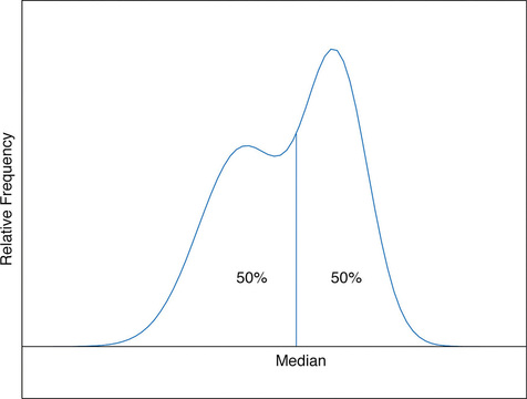
The median is a value that divides the observations in a data set so that \(50\%\) of the data are on its left and the other \(50\%\) on its right. In accordance with Figure \(\PageIndex{7}\), therefore, in the curve that represents the distribution of the data, a vertical line drawn at the median divides the area in two, area \(0.5\) (\(50\%\) of the total area \(1\)) to the left and area \(0.5\) (\(50\%\) of the total area \(1\)) to the right, as shown in Figure \(\PageIndex{1}\). In our income example the median, \($24,600\), clearly gave a much better measure of the middle of the data set than did the mean \($47,400\). This is typical for situations in which the distribution is skewed. (Skewness and symmetry of distributions are discussed at the end of this subsection.)
Compute the sample median for the data from Example \(\PageIndex{2}\)
Solution
The data in numerical order are \(−1, 0, 2, 2\). The two middle measurements are \(0\) and \(2\), so \(\tilde{x}= (0+2)/2 = 1\).
Compute the sample median for the data from Example \(\PageIndex{3}\)
Solution
The data in numerical order are
The number of observations is ten, which is even, so there are two middle measurements, the fifth and sixth, which are \(2.53\) and \(2.71\). Therefore the median of these data is \(\tilde{x} = (2.53+2.71)/2 = 2.62\).
Compute the sample median for the data from Example \(\PageIndex{4}\)
Solution
The data in numerical order are:
The number of observations is \(19\), which is odd, so there is one middle measurement, the tenth. Since the tenth measurement is \(2\), the median is \(\tilde{x} = 2\).
In the last example it is important to note that we could have computed the median directly from the frequency table, without first explicitly listing all the observations in the data set. We already saw in Example \(\PageIndex{4}\) how to find the number of observations directly from the frequencies listed in the table \(n = 3+6+6+3+1 = 19\). Thus the median is the tenth observation. The second line of the table in Example \(\PageIndex{4}\) shows that when the data are listed in order there will be three \(0s\) followed by six \(1s\), so the tenth observation, the median, is \(2\).
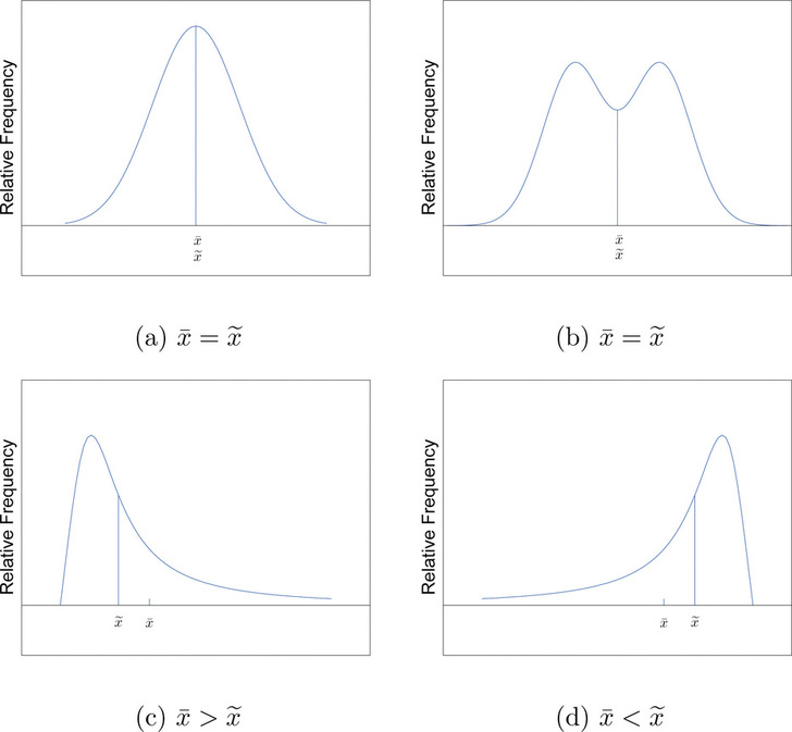
The relationship between the mean and the median for several common shapes of distributions is shown in Figure \(\PageIndex{2}\). The distributions in panels (a) and (b) are said to be symmetric because of the symmetry that they exhibit. The distributions in the remaining two panels are said to be skewed. In each distribution we have drawn a vertical line that divides the area under the curve in half, which in accordance with Figure \(\PageIndex{1}\) is located at the median. The following facts are true in general:
- When the distribution is symmetric, as in panels (a) and (b) of Figure \(\PageIndex{2}\), the mean and the median are equal.
- When the distribution is as shown in panel (c), it is said to be skewed right. The mean has been pulled to the right of the median by the long “right tail” of the distribution, the few relatively large data values.
- When the distribution is as shown in panel (d), it is said to be skewed left. The mean has been pulled to the left of the median by the long “left tail” of the distribution, the few relatively small data values.
The Mode
Perhaps you have heard a statement like “The average number of automobiles owned by households in the United States is \(1.37\),” and have been amused at the thought of a fraction of an automobile sitting in a driveway. In such a context the following measure for central location might make more sense.
The sample mode of a set of sample data is the most frequently occurring value.
On a relative frequency histogram, the highest point of the histogram corresponds to the mode of the data set. Figure \(\PageIndex{3}\) illustrates the mode.
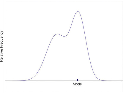
Figure \(\PageIndex{3}\): Mode
For any data set there is always exactly one mean and exactly one median. This need not be true of the mode; several different values could occur with the highest frequency, as we will see. It could even happen that every value occurs with the same frequency, in which case the concept of the mode does not make much sense.
Find the mode of the following data set: \(-1,\; 0,\; 2,\; 0\).
Solution
The value \(0\) is most frequently observed in the data set, so the mode is \(0\).
Compute the sample mode for the data of Example \(\PageIndex{4}\)
Solution
The two most frequently observed values in the data set are \(1\) and \(2\). Therefore mode is a set of two values: \(\{1,2\}\).
The mode is a measure of central location since most real-life data sets have more observations near the center of the data range and fewer observations on the lower and upper ends. The value with the highest frequency is often in the middle of the data range.
Key Takeaway
- The mean, the median, and the mode each answer the question “Where is the center of the data set?” The nature of the data set, as indicated by a relative frequency histogram, determines which one gives the best answer.