
15.3.2: Chapter 3 Lab
- Page ID
- 28616

\( \newcommand{\vecs}[1]{\overset { \scriptstyle \rightharpoonup} {\mathbf{#1}} } \) \( \newcommand{\vecd}[1]{\overset{-\!-\!\rightharpoonup}{\vphantom{a}\smash {#1}}} \)\(\newcommand{\id}{\mathrm{id}}\) \( \newcommand{\Span}{\mathrm{span}}\) \( \newcommand{\kernel}{\mathrm{null}\,}\) \( \newcommand{\range}{\mathrm{range}\,}\) \( \newcommand{\RealPart}{\mathrm{Re}}\) \( \newcommand{\ImaginaryPart}{\mathrm{Im}}\) \( \newcommand{\Argument}{\mathrm{Arg}}\) \( \newcommand{\norm}[1]{\| #1 \|}\) \( \newcommand{\inner}[2]{\langle #1, #2 \rangle}\) \( \newcommand{\Span}{\mathrm{span}}\) \(\newcommand{\id}{\mathrm{id}}\) \( \newcommand{\Span}{\mathrm{span}}\) \( \newcommand{\kernel}{\mathrm{null}\,}\) \( \newcommand{\range}{\mathrm{range}\,}\) \( \newcommand{\RealPart}{\mathrm{Re}}\) \( \newcommand{\ImaginaryPart}{\mathrm{Im}}\) \( \newcommand{\Argument}{\mathrm{Arg}}\) \( \newcommand{\norm}[1]{\| #1 \|}\) \( \newcommand{\inner}[2]{\langle #1, #2 \rangle}\) \( \newcommand{\Span}{\mathrm{span}}\)\(\newcommand{\AA}{\unicode[.8,0]{x212B}}\)
Descriptive Statistics (Chapter 1, 2 required)
Open MINITAB file lab02.mpj from the website. This data represents information 700 instructors from the popular website ratemyprofessors.com. All instructors are sampled from the Foothill‐De Anza Community College District. Here is a description of the data:
| College | Foothill or De Anza |
| Smiley |  Positive Positive  Neutral Neutral  Negative Negative |
| Photo | Instructor has a photo |
| Hot |  Instructor has a chili pepper Instructor has a chili pepper |
| Gender | Male or Female |
| Dept | Academic Department (example ‐ Mathematics) |
| Division | Academic Division (example ‐ PSME) |
| Num | Number of Ratings for that faculty member |
| Overall | Average Overall Quality Rating (1‐5 scale, lowest to highest) |
| Easiness | Average Easiness Rating (1‐5 scale, hardest to easiest) |
In Lab 1, we constructed some dot plots and made some interpretations of Average Overall Quality Rating. In Lab 2, we will look at other graphs and statistics that measure center, spread and relative standing.
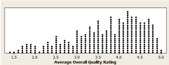
- Above is a dot plot you made of Average Overall Quality Rating in Lab 1. Make a histogram of the Average Overall Quality Rating. Paste the graph here. Are both graphs showing the same center, spread and shape? Explain your answer. Descriptive Statistics can be found in Minitab under STAT>BASIC STATISTICS.
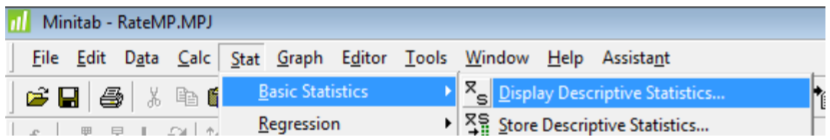
- Use this command to determine the sample mean and sample median for the Average Overall Quality Rating. Paste the results here and answer these questions:
- Which statistic is a better measure of center for this data? Explain your answer.
- Are the values of the sample mean and median consistent with the shape of the histogram? Explain your answer.
Here are dot plots comparing Average Overall Quality Ratings of instructors who are rated "hot" vs. those who are rated "not hot"; these plots were made in Lab 1.
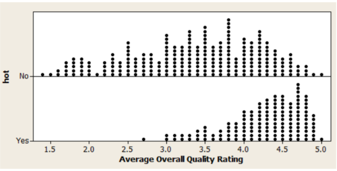
- Under the GRAPHS menu bar in Minitab, create box plots of Average Overall Quality Ratings comparing "hot" and "not hot" instructors. Paste the results here and from the box plots, answer these questions.
- Which group has a higher sample median?
- For the "hot" instructors, between what values would you find the middle 50% of ratings?
- For the "not hot" instructors, between what values would you find the middle 50% of ratings?
- Are there any possible outliers for the "hot" instructors? Explain.
- Under the STAT>BASIC STATISTICS menu, find descriptive statistics of overall ratings for both "hot" and "not hot" instructors. Paste the results here. Then answer the following questions:
- Which group has a higher sample mean? Is this result consistent with your box plot?
- Which group has a higher sample standard deviation? Is this result consistent with your box plot?
- What is more unusual: a "hot" instructor with an Overall Rating of 3.5 or a "not hot" instructor with an Overall Rating of 3.5? Calculate and compare the Z‐scores for each instructor to answer this question.
- Using the Empirical Rule, between what two Average Overall Quality Ratings would you find 68% of the "not hot" instructors?
- Under the STAT>BASIC STATISTICS menu, find descriptive statistics of overall ratings split by college for both "Foothill" and "De Anza" instructors. Paste the results here. Then answer the following questions:
- Which group has a higher sample mean? Is this result consistent with your box plot?
- Which group has a higher sample standard deviation? Is this result consistent with your box plot?
- What is more unusual: a "Foothill" instructor with an Overall Rating of 2.3 or a "De Anza" instructor with an Overall Rating of 2.3? Calculate and compare the Z‐scores for each instructor to answer this question.
- Using the Empirical Rule, between what two Average Overall Quality Ratings would you find 68% of the "De Anza" instructors?
- To make a scatterplot: MINITAB>GRAPHS>SCATTERPLOT To find correlation coefficients: MINITAB> BASIC STATISTICS>CORRELATION
- Create a scatterplot in which the dependent variable is Overall and the independent variable is Num. Paste the graph here. Describe the strength, direction and linearity of the correlation.
- Determine the correlation coefficient of Overall and Num. Is the result consistent with part a?
- Create a scatterplot in which the dependent variable is Overall and the independent variable is Easiness. Paste the graph here. Describe the strength, direction and linearity of the correlation.
- Determine the correlation coefficient of Overall and Easiness. Is the result consistent with part c? Why are these two variables correlated? Give at least two possible explanations.