14.9: Residual Analysis

Last updated
Save as PDF

Page ID: 20934

\( \newcommand{\vecs}[1]{\overset { \scriptstyle \rightharpoonup} {\mathbf{#1}} } \) \( \newcommand{\vecd}[1]{\overset{-\!-\!\rightharpoonup}{\vphantom{a}\smash {#1}}} \)\(\newcommand{\id}{\mathrm{id}}\) \( \newcommand{\Span}{\mathrm{span}}\) \( \newcommand{\kernel}{\mathrm{null}\,}\) \( \newcommand{\range}{\mathrm{range}\,}\) \( \newcommand{\RealPart}{\mathrm{Re}}\) \( \newcommand{\ImaginaryPart}{\mathrm{Im}}\) \( \newcommand{\Argument}{\mathrm{Arg}}\) \( \newcommand{\norm}[1]{\| #1 \|}\) \( \newcommand{\inner}[2]{\langle #1, #2 \rangle}\) \( \newcommand{\Span}{\mathrm{span}}\) \(\newcommand{\id}{\mathrm{id}}\) \( \newcommand{\Span}{\mathrm{span}}\) \( \newcommand{\kernel}{\mathrm{null}\,}\) \( \newcommand{\range}{\mathrm{range}\,}\) \( \newcommand{\RealPart}{\mathrm{Re}}\) \( \newcommand{\ImaginaryPart}{\mathrm{Im}}\) \( \newcommand{\Argument}{\mathrm{Arg}}\) \( \newcommand{\norm}[1]{\| #1 \|}\) \( \newcommand{\inner}[2]{\langle #1, #2 \rangle}\) \( \newcommand{\Span}{\mathrm{span}}\)\(\newcommand{\AA}{\unicode[.8,0]{x212B}}\)

In regression, we assume that the model is linear and that the residual errors (\(Y-\hat{Y}\) for each pair) are random and normally distributed. We can analyze the residuals to see if these assumptions are valid and if there are any potential outliers. In particular:

The residuals should represent a linear model.
The standard error (standard deviation of the residuals) should not change when the value of \(X\) changes.
The residuals should follow a normal distribution.
Look for any potential extreme values of \(X\).
Look for any extreme residual errors.

Example: Model A

Model A is an example of an appropriate linear regression model. We will make three graphs to test the residual; a scatterplot with the regression line, a plot of the residuals, and a histogram of the residuals

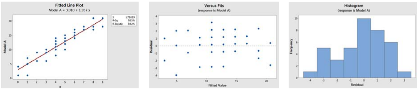
Here we can see the that residuals appear to be random, the fit is linear, and the histogram is approximately bell shaped. In addition, there are no extreme outlier values of \(X\) or outlier residuals.

Example: Model B

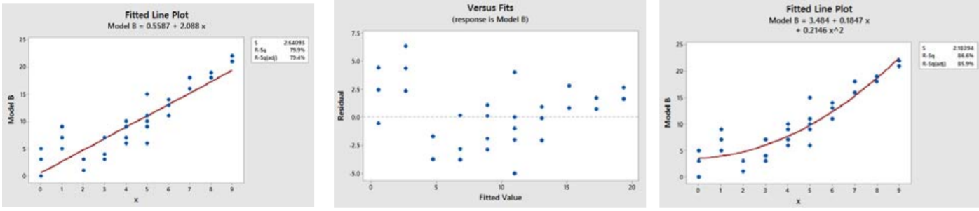
Model B looks like a strong fit, but the residuals are showing a pattern of being positive for low and high values of \(X\) and negative for middle values of \(X\). This indicates that the model is not linear and should be fit with a non‐linear regression model (for example, the third graph shows a quadratic model).

Example: Model C

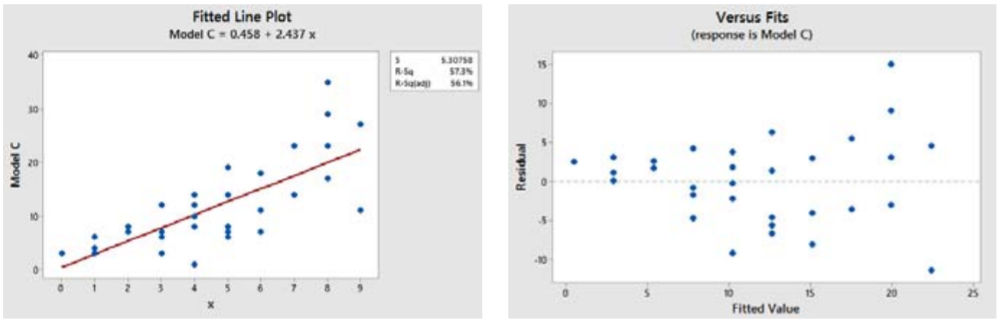
Model C has a linear fit, but the residuals are showing a pattern of being smaller for low values of \(X\) and higher for large values of \(X\). This violates the assumption that the standard error should not change when the value of \(X\) changes. This phenomena is called heteroscedasticity and requires a data transformation to find a more appropriate model.

Example: Model D

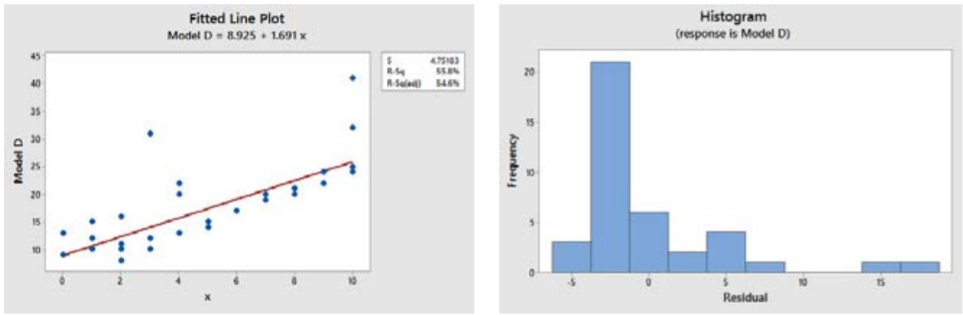
Model D seems to have a linear fit, but the residuals are showing a pattern of being larger when they are positive and smaller when they are negative. This violates the assumption that residuals should follow a normal distribution, as can be seen in the histogram.

Example: Model E

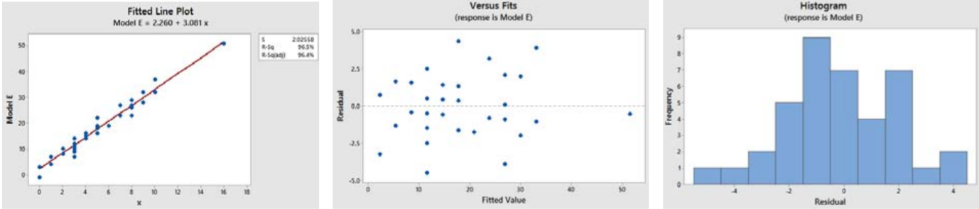
Model E seems to have a linear fit, and the residuals look random and normal. However, the value (16,51) is an extreme outlier value of \(X\) and may have an undue influence on the choosing of the regression line.

Example: Model F

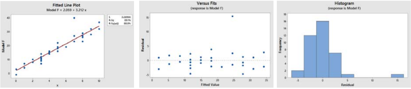
Model F seems to have a linear fit, and the residuals look random and normal, except for one outlier at the value (7,40). This outlier is different than the extreme outlier in Model E, but will still have an undue influence on the choosing of the regression line.