13.6: Post‐hoc Analysis – Tukey’s Honestly Significant Difference (HSD) Test85

Last updated
Save as PDF

Page ID: 20925

\( \newcommand{\vecs}[1]{\overset { \scriptstyle \rightharpoonup} {\mathbf{#1}} } \) \( \newcommand{\vecd}[1]{\overset{-\!-\!\rightharpoonup}{\vphantom{a}\smash {#1}}} \)\(\newcommand{\id}{\mathrm{id}}\) \( \newcommand{\Span}{\mathrm{span}}\) \( \newcommand{\kernel}{\mathrm{null}\,}\) \( \newcommand{\range}{\mathrm{range}\,}\) \( \newcommand{\RealPart}{\mathrm{Re}}\) \( \newcommand{\ImaginaryPart}{\mathrm{Im}}\) \( \newcommand{\Argument}{\mathrm{Arg}}\) \( \newcommand{\norm}[1]{\| #1 \|}\) \( \newcommand{\inner}[2]{\langle #1, #2 \rangle}\) \( \newcommand{\Span}{\mathrm{span}}\) \(\newcommand{\id}{\mathrm{id}}\) \( \newcommand{\Span}{\mathrm{span}}\) \( \newcommand{\kernel}{\mathrm{null}\,}\) \( \newcommand{\range}{\mathrm{range}\,}\) \( \newcommand{\RealPart}{\mathrm{Re}}\) \( \newcommand{\ImaginaryPart}{\mathrm{Im}}\) \( \newcommand{\Argument}{\mathrm{Arg}}\) \( \newcommand{\norm}[1]{\| #1 \|}\) \( \newcommand{\inner}[2]{\langle #1, #2 \rangle}\) \( \newcommand{\Span}{\mathrm{span}}\)\(\newcommand{\AA}{\unicode[.8,0]{x212B}}\)

When the Null Hypothesis is rejected in one factor ANOVA, the conclusion is that not all means are the same. This however leads to an obvious question: which particular means are different? Seeking further information after the results of a test is called post‐hoc analysis.

The problem of multiple tests

One attempt to answer this question is to conduct multiple pairwise independent same t‐tests and determine which ones are significant. We would compare \(\mu_{1}\) to \(\mu_{2}\), \(\mu_{1}\) to \(\mu_{3}\), \(\mu_{2}\) to \(\mu_{3}\), \(\mu_{1}\) to \(\mu_{4}\), etc. There is a major flaw in this methodology in that each test would have a significance level of \(\alpha\), so making Type I error would be significantly more than the desired \(\alpha\). Furthermore, these pairwise tests would NOT be mutually independent. There were several statisticians who designed tests that effectively dealt with this problem of determining an "honest" significance level of a set of tests; we will cover the one developed by John Tukey, the Honestly Significant Difference (HSD) test.⁸⁶ To use this test, we need the critical value from the Studentized Range Distribution (\(q\)), which is used to find when difference of pairs of sample means are significant.

The Tukey HSD test

Tests: \(H_{o}: \mu_{i}=\mu_{j} \quad H_{a}: \mu_{i} \neq \mu_{j}\) where the subscripts \(i\) and \(j\) represent two different populations

Overall significance level of \(\alpha\): This means that all pairwise tests can be run at the same time with an overall significance level of \(\alpha\)

Test Statistic: \(\mathrm{HSD}=q \sqrt{\dfrac{\mathrm{MSE}{n_{c}}}\)

\(q\) = critical value from Studentized Range table

\(\mathrm{MSE}\) = Mean Square Error from ANOVA table

\(n_c\) = number of replicates per treatment. An adjustment is made for unbalanced designs.

Decision: Reject \(H_o\) if \(\left|\overline{X}_{i}-\overline{X}_{j}\right|>\mathrm{HSD}_\text{critical value}\)

Computer software, such as Minitab, will calculate the critical values and test statistics for these series of tests. We will not perform the manual calculations in this text.

Example: Party Pizza

Let us return to the Tofu pizza example where we rejected the Null Hypothesis and supported the claim that there was a difference in means among the three restaurants.

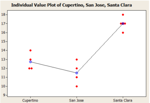
In reviewing the graph of the sample means, it appears that Santa Clara has a much higher number of sales than Cupertino and San Jose. There will be three pairwise post‐hoc tests to run.

Solution

Design

\(H_{o}: \mu_{1}=\mu_{2} \qquad H_{a}: \mu_{1} \neq \mu_{2} \qquad H_{o}: \mu_{1}=\mu_{3} \qquad H_{a}: \mu_{1} \neq \mu_{3} \qquad H_{o}: \mu_{2}=\mu_{3} \qquad H_{a}: \mu_{2} \neq \mu_{3}\)

These three tests will be conducted with an overall significance level of \(\alpha\) = 5%.

The model will be the Tukey \(\mathrm{HSD}\) test.

Here are the differences of the sample means for each pair ranked from lowest to highest:

Test 1: Cupertino to San Jose: \(\left|\overline{X}_{1}-\overline{X}_{2}\right|=|12.75-11.50|=1.25\)

Test 2: Cupertino to Santa Clara: \(\left|\overline{X}_{1}-\overline{X}_{3}\right|=|12.75-17.00|=4.25\)

Test 3: San Jose to Santa Clara: \(\left|\overline{X}_{2}-\overline{X}_{3}\right|=|11.50-17.00|=5.50\)

The \(\mathrm{HSD}\) critical values (using statistical software) for this particular test:

\(\mathrm{HSD}_\text{crit}\) at 5% significance level = 1.85 \(\mathrm{HSD}_\text{crit}\) at 1% significance level = 2.51

For each test, reject \(H_o\) if the difference of means is greater than \(\mathrm{HSD}_\text{crit}\)

Test 2 and Test 3 show significantly different means at both the 1% and 5% level.

The Minitab approach for the decision rule will be to reject \(H_o\) for each pair that does not share a common group. Here are the results for the test conducted at the 5% level of significance:

Data/Results

Refer to the Minitab output. Santa Clara is in group A while Cupertino and San Jose are in Group B.

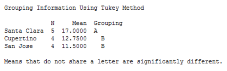
Conclusion

Santa Clara has a significantly higher mean number of tofu pizzas sold compared to both San Jose and Cupertino. There is no significant difference in mean sales between San Jose and Cupertino.