
13.5: Understanding the ANOVA Table
- Page ID
- 20924

When running Analysis of Variance, the data is usually organized into a special ANOVA table, especially when using computer software.
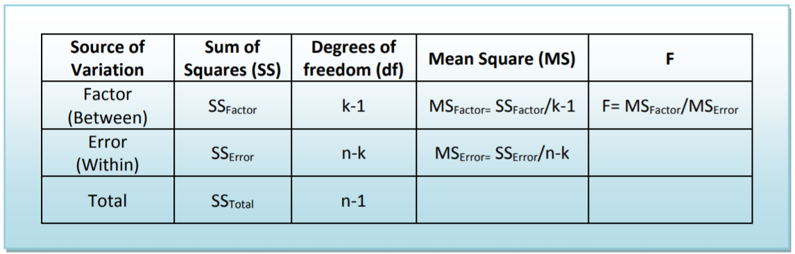
Sum of Squares: The total variability of the numeric data being compared is broken into the variability between groups (\(\mathrm{SS}_{\text {Factor }}\)) and the variability within groups (\(\mathrm{SS}_{\text {Error }}\)). These formulas are the most tedious part of the calculation. \(T_c\) represents the sum of the data in each population and \(n_c\) represents the sample size of each population. These formulas represent the numerator of the variance formula.
\[\mathrm{SS}_{\text {Total }}=\Sigma\left(X^{2}\right)-\dfrac{(\Sigma X)^{2}}{n} \nonumber \]
\[\mathrm{SS}_{\text {Factor }}=\Sigma\left(\dfrac{T_{c}^{2}}{n_{c}}\right)-\dfrac{(\Sigma X)^{2}}{n} \nonumber \]
\[\mathrm{SS}_{\text {Error }}=\mathrm{SS}_{\text {Total }}-\mathrm{SS}_{\text {Factor }} \nonumber \]
Degrees of freedom: The total degrees of freedom is also partitioned into the Factor and Error components.
Mean Square: This represents calculation of the variance by dividing Sum of Squares by the appropriate degrees of freedom.
\(\mathrm{F}\): This is the test statistic for ANOVA: the ratio of two sample variances (mean squares) that are both estimating the same population value has an \(\mathrm{F}\) distribution. Computer software will then calculate the \(p\)‐ value to be used in testing the Null Hypothesis that all populations have the same mean.
Party Pizza specializes in meals for students. Hsieh Li, President, recently developed a new tofu pizza.

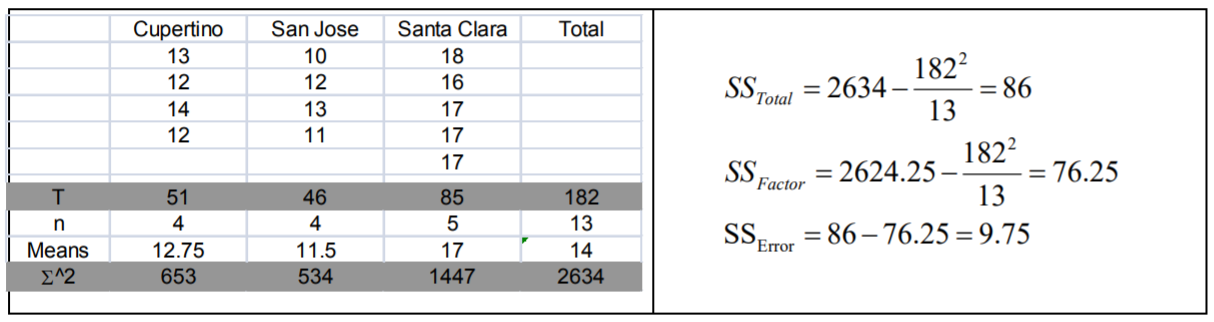
Before making it a part of the regular menu she decides to test it in several of her restaurants. She would like to know if there is a difference in the mean number of tofu pizzas sold per day at the Cupertino, San Jose, and Santa Clara pizzerias. Data will be collected for five days at each location.
At the .05 significance level can Hsieh Li conclude that there is a difference in the mean number of tofu pizzas sold per day at the three pizzerias?
Solution
Design
Response: tofu pizzas sold
Factor: location of restaurant
Levels: \(k = 3\) (Cupertino, San Jose, Santa Clara)
Research Hypotheses:
\(H_o\): There is no difference in mean tofu pizzas sold due to location of restaurant.
\(H_a\): There is a difference in mean tofu pizzas sold due to location of restaurant
\(H_o\): \(\mu_{1}=\mu_{2}=\mu_{3}\) (Mean sales same at all restaurants)
\(H_a\): At least \(\mu_{i}\) is different (Means sales not the same at all restaurants)
We will assume the population variances are equal \(\sigma_{1}^{2}=\sigma_{2}^{2}=\sigma_{3}^{2}\), so the model will be One Factor ANOVA. This model is appropriate if the distribution of the sample means is approximately Normal from the Central Limit Theorem.
Type I error would be to reject the Null Hypothesis and claim mean sales are different, when they actually are the same. The test will be run at a level of significance (\(\alpha\)) of 5%.
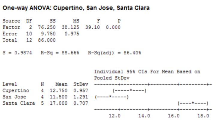
The test statistic from the table will be \(\mathrm{F}=\dfrac{\mathrm {MS}_\text{Factor }}{\mathrm {MS}_\text{Error }}\). The degrees of freedom for numerator will be 3‐1=2,and the degrees of freedom for denominator will be 13‐3=10. (The total sample size turned out to be only 13, not 15 as planned).
Critical Value for \(\mathrm{F}\) at \(\alpha\) of 5% with \(\mathrm{df}_{\text {num }}=2\) and \(\mathrm{df}_{\text {den }}=10\) is 4.10. Reject \(H_o\) if \(\mathrm{F}\) >4.10. We will also run this test using the p‐value method with statistical software, such as Minitab.
Data/Results
\(\mathrm{F}=38.125 / 0.975=39.10\), which is more than the critical value of 4.10, so reject \(H_o\). Also from the Minitab output, \(p\)‐value = 0.000 < 0.05 which also supports rejecting \(H_o\).
Conclusion
There is a difference in the mean number of tofu pizzas sold at the three locations.