
12.1: Chi‐square Goodness‐of‐fit Test
- Page ID
- 20918

A financial services company had anecdotal evidence that people were calling in sick on Monday and Friday more frequently than on Tuesday, Wednesday or Thursday. The speculation was that some employees were using sick days to extend their weekends. A researcher for the company was asked to determine if the data supported a significant difference in absenteeism due to the day of the week.
The categorical variable of interest here is “Day of Week” an employee called in sick (Monday through Friday). This is an example of a multinomial random variable, in which we will observe a fixed number of trials (the total number of sick days sampled) and at least 2 possible outcomes. (A binomial random variable is a special case of the multinomial random variable where there is exactly 2 possible outcomes and was studied in Chapter 10 as a \(Z\) Test of Proportion.)
The Chi‐square goodness‐of‐fit test is used to test if observed data from a categorical variable is consistent with an expected assumption about the distribution of that variable.
Model Assumptions
- \(O_{i}\) = Observed in category \(i\)
- \(p_{i}\) = Expected proportion in category \(i\)
- \(E_{i}=n p_{i}\) = Expected in category \(i\)
- \(E_{i} \geq 5\) for each \(i\)
Test Statistic
\(\chi^{2}=\sum_{i=1}^{k} \dfrac{\left(O_{i}-E_{i}\right)^{2}}{E_{i}} \quad \mathrm{df}=k-1\) where
\(k\) = number of categories \(n\) = sample size
Chi‐Square Goodness‐of‐Fit test ‐ equal expected frequencies
Example: Sick days

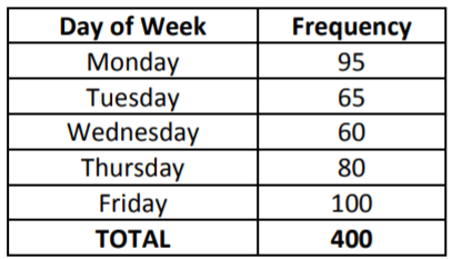
A researcher for the financial services company collected 400 records of which day of the week employees called in sick to work. Can the researcher conclude that proportion of employees who call in sick is not the same for each day of the week? Design and conduct a hypothesis test at the 1% significance level.
Solution
Research Hypotheses:
\(H_o\): There is a no difference in the proportion of employees who call in sick due to the day of the week.
\(H_a\): There is a difference in the proportion of employees who call in sick due to the day of the week.
We can also state the hypotheses in terms of population parameters, \(p_i\) for each category. Under the Null Hypothesis, we would expect 20% sick days would occur on each week day.
Research Hypotheses:
\(H_o: p_{1}=p_{2}=p_{3}=p_{4}=p_{5}=0.20\)
\(H_a\): At least one pi is different than what was stated in \(H_o\)
Statistical Model: Chi‐square goodness‐of‐fit test.
Important Assumption: The Expected Value of Each Category needs to be greater than or equal to 5. In this example, \(E_{i}=n p_{i}=(400)(.20)=80 \geq 5\) for each category, so the model is appropriate.
Test Statistic: \(\chi^{2}=\sum_{i=1}^{k} \dfrac{\left(O_{i}-E_{i}\right)^{2}}{E_{i}} \qquad \mathrm{df}=5-1=4\)
Decision Rule (Critical Value Method): Reject \(H_o\) if \(\chi^{2}>13.277 (\alpha=.01, 4 \mathrm{df})\)
Results:
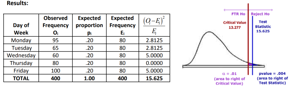
Since the Test Statistic is in the Rejection Region, the decision is to Reject \(H_o\). Under the \(p\)‐value method, \(H_o\) is also rejected since the \(p \text {-value }=p\left(\chi^{2}>15.625\right)=0.004\), which is less than the Significance Level \(\alpha\) of 1%.
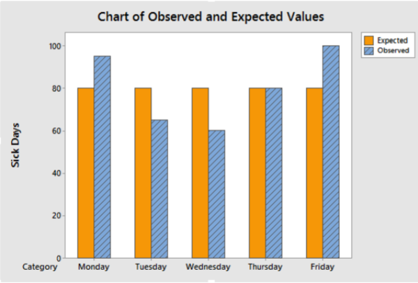
Conclusion:
There is a difference in the proportion of employees who call in sick due to the day of the week. Employees are more likely to call in sick on days close to the weekend.
Chi‐Square Goodness‐of‐Fit test ‐ different expected frequencies
In the prior example, the Null Hypothesis was that all categories had the same proportion; in other words, there was no difference in counts due to the choices of a categorical variable. Another set of hypotheses using this same Chi‐square goodness‐of‐fit test can be used to compare current results of a current experiment to prior results. In these tests, it is quite likely that prior proportions were not the same.
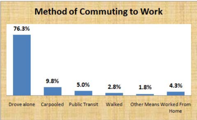
Example: Method of Commuting)
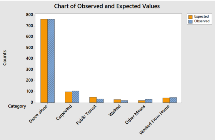
In the 2010 United States census, data was collected on how people get to work ‐‐ their method of commuting. The results are shown in the graph to the right. Suppose you wanted to know if people who live in the San Jose metropolitan area (Santa Clara County) commute with similar proportions as the United States. We will sample 1000 workers from Santa Clara County and conduct a Chi‐square goodness‐of‐fit test. Design and conduct a hypothesis test at the 5% significance level.
Solution
Research Hypotheses:
\(H_o\): Workers in Santa Clara county choose methods of commuting that match the United States averages.
\(H_a\): Workers in Santa Clara county choose methods of commuting that do not match the United States averages.
We can also state the hypotheses in terms of population parameters, \(p_i\) for each category. Under the Null Hypothesis, we would expect the Santa Clara proportions to be the same as the US 2010 Census data.
Research Hypotheses:
\(H_o: p_{1}=.763 p_{2}=.098 p_{3}=.050 p_{4}=.028 p_{5}=.018 p_{6}=.043\)
\(H_a\): At least one \(p_i\) is different than what was stated in \(H_o\)
Statistical Model: Chi‐square goodness‐of‐fit test.
Important Assumption: The Expected Value of Each Category needs to be greater than or equal to 5. In this example check the lowest \(p_{i}: E_{5}=n p_{5}=(1000)(.018)=18 \geq 5\), so the model is appropriate.
Test Statistic: \(\chi^{2}=\sum_{i=1}^{k} \dfrac{\left(O_{i}-E_{i}\right)^{2}}{E_{i}} \qquad \mathrm{df}=6-1=5\)
Decision Rule (Critical Value Method): Reject \(H_o\) if \(\chi^{2}>11.071 (\alpha=.05, 5 \mathrm{df})\)
After designing the experiment, we conducted the sample of Santa Clara County, shown in the Observed Frequency Column of the table below. The Expected Proportion and Expected Frequency Columns are calculated using the U.S. 2010 Census.
Results:
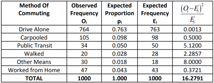
Since the Test Statistic of 16.2791 exceeds the critical value of 11.071, the decision is to Reject \(H_o\). Under the \(p\)‐value method, \(H_o\) is also rejected since the \(p \text {-value }=P\left(\chi^{2}>16.2791\right)=0.006\) which is less than the Significance Level \(\alpha\) of 5%.
Conclusion:
Workers in Santa Clara County do not have the same frequencies of method of commuting as workers in the entire United States.