9.3: Confidence Intervals

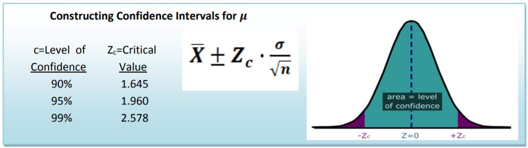
Using probability and the Central Limit Theorem, we can design an Interval Estimate called a Confidence Interval which has a known probability (Level of Confidence) of capturing the true population parameter.

Confidence Interval for Population Mean

To find a confidence interval for the population mean (\(\mu\)) when the population standard deviation (\(\sigma\))is known, and n is sufficiently large, we can use the Standard Normal Distribution probability distribution function to calculate the critical values for the Level of Confidence:  

Example: Students working

The Dean wants to estimate the mean number of hours that students worked per week.  A sample of 49 students showed a mean of 24 hours with a standard deviation of 4 hours. The point estimate is 24 hours (sample mean). What is the 95% confidence interval for the average number of hours worked per week by the students?

Solution

\[24 \pm \dfrac{1.96 \cdot 4}{\sqrt{49}}=24 \pm 1.12=(22.88,25.12) \text{ hours per week} \nonumber \]

The margin of error for the confidence interval is 1.12 hours. We can say with 95% confidence that the mean number of hours worked by students is between 22.88 and 25.12 hours per week.

If the level of confidence is increased, then the margin of error will also increase. For example, if we increase the level of confidence to 99% for the above example, then:

\[24 \pm \dfrac{2.578 \cdot 4}{\sqrt{49}}=24 \pm 1.47=(22.53,25.47) \text{ hours per week} \nonumber \]

Some important points about Confidence Intervals

• The confidence interval is constructed from random variables calculated from sample data and attempts to predict an unknown but fixed population parameter with  a certain level of confidence.  
• Increasing the level of confidence will always increase the margin of error.
• It is impossible to construct a 100% Confidence Interval without taking a census of the entire population.
• Think of the population mean as a dart that always goes to the same spot, and the confidence interval as a moving target that tries to “catch the dart.” A 95% confidence interval would be like a target that has a 95% chance of catching the dart. 

Confidence Interval for Population Mean using Sample Standard Deviation – Student’s t Distribution

The formula for the confidence interval for the mean requires the knowledge of the population standard deviation (\(\sigma\)). In most real‐life problems, we do not know this value for the same reasons that we do not know the population mean. This problem was solved by the Irish statistician William Sealy Gosset, an employee at Guinness Brewing. Gosset, however, was prohibited by Guinness from using his own name in publishing scientific papers. He published under the name “A Student”, and therefore the distribution he discovered was named "Student's \(t\)‐distribution"⁷¹.

Characteristics of Student’s t Distribution

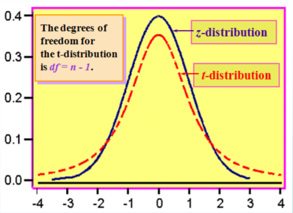
• It is continuous, bell‐shaped, and symmetrical about zero like the \(z\) distribution.
• There is a family of \(t\)‐distributions sharing a mean of zero but having different standard deviations based on degrees of freedom.
• The \(t\)‐distribution is more spread out and flatter at the center than the \(Z\)‐distribution, but approaches the \(Z\)‐distribution as the sample size gets larger.   

Confidence Interval for \(\mu\)

\[\overline{X} \pm t_{c} \dfrac{s}{\sqrt{n}} \text{ with degrees of freedom} = n - 1 \nonumber \]

Example: Rating heath care plans

Last year Sally belonged to an Health Maintenance Organization (HMO) heath care plan that had a population average rating of 62 (on a scale from 0‐100, with ‘100’ being best); this was based on records accumulated about the HMO over a long period of time. This year Sally switched to a new HMO.  To assess the population mean rating of the new HMO, 20 members of this HMO are polled and they give the HMO  an average rating of 65 with a standard deviation of 10. Find and interpret a 95% confidence interval for population average rating of the new HMO.

Solution

The \(t\) distribution will have 20‐1 =19 degrees of freedom. Using a table or technology, the critical value for the 95%  confidence interval will be  \(t_c=2.093\)

\[65 \pm \dfrac{2.093 \cdot 10}{\sqrt{20}}=65 \pm 4.68=(60.32,69.68) \text{ HMO rating} \nonumber \]

With 95% confidence we can say that the rating of Sally’s new HMO is between 60.32 and 69.68. Since the quantity 62 is in the confidence interval, we cannot say with 95% certainty that the new HMO is either better or worse than the previous HMO.

Confidence Interval for Population Proportion

Recall from the section on random variables the binomial distribution where \(p\) represented the proportion of successes in the population. The binomial model was analogous to coin‐flipping, or yes/no question polling. In practice, we want to use sample statistics to estimate the population proportion (\(p\)).

The sample proportion (\(\hat{p}\)) is the proportion of successes in the sample of size \(n\) and is the point estimator for \(p\). Under the Central Limit Theorem, if \(n p>10\) and \(n(1-p)>10\), the distribution of the sample proportion \(\hat{p}\) will have an approximately Normal Distribution.

Normal Distribution for \(\hat{p}\) if Central Limit Theorem conditions are met.

\[\mu_{\hat{p}}=p \qquad \qquad \sigma_{\hat{p}}=\sqrt{\dfrac{p(1-p)}{n}} \nonumber \]

Using this information we can construct a confidence interval for \(p\), the population proportion:

Confidence interval for \(p\)

\[\hat{p} \pm Z \sqrt{\dfrac{p(1-p)}{n}} \approx \hat{p} \pm Z \sqrt{\frac{\hat{p}(1-\hat{p})}{n}} \nonumber \]

Example: Talking and driving

200 California drivers were randomly sampled and it was discovered that 25 of these drivers were illegally talking on their cell phones without the use of a hands‐free device. Find the point estimator for the proportion of drivers who are using their cell phones illegally and construct a 99% confidence interval.

Solution

The point estimator for \(p\) is \(\hat{p}=\dfrac{25}{200}=.125\) or 12.5%.

A 99% confidence interval for \(p\) is: \(0.125 \pm 2.576 \sqrt{\dfrac{.125(1-.125)}{200}}=.125 \pm .060\)

The margin of error for this poll is 6% and we can say with 99% confidence that the true percentage of drivers who are using their cell phones illegally is between 6.5% and 18.5%

Point Estimator for Population Standard Deviation 

We often want to study the variability, volatility or consistency of a population. For example, two investments both have expected earnings of 6% per year, but one investment is much riskier, with higher ups and downs. To estimate variation or volatility of a data set, we will use the sample standard deviation \(s\) as a point estimator of the population standard deviation (\(\sigma\)).

Example

Investments A and B are both known to have a rate of return of 6% per year. Over the last 24 months, Investment A has a sample standard deviation of 3% per month, while Investment B has a sample standard deviation of 5% per month.  We would say that Investment B is more volatile and riskier than Investment A due to the higher estimate of the standard deviation.

To create a confidence interval for an estimate of standard deviation, we need to introduce a new distribution, called the Chi‐square (\(\chi^{2}\)) distribution.

The Chi‐square \(\chi^{2}\) Distribution

The Chi‐square distribution is a family of distributions related to the Normal Distribution, since it represents a sum of independent squared standard Normal Random Variables. Like the Student’s t distribution, the degrees of freedom will be \(n - 1\) and will determine the shape of the distribution. Also, since the Chi‐square represents squared data, the inference will be about the variance rather than about the standard deviation.  

Characteristics of Chi‐square \(\chi^{2}\) Distribution

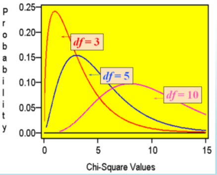
• It is positively skewed
• It is non‐negative
• It is based on degrees of freedom (\(n - 1\))
• When the degrees of freedom change, a new distribution is created \(\dfrac{(n-1) s^{2}}{\sigma^{2}}\) will have Chi‐square distribution.

Confidence Interval for Population Variance and Standard Deviation

Since the Chi‐square represents squared data, we can construct confidence intervals for the population variance (\(\sigma^{2}\)), and take the square root of the endpoints to get a confidence interval for the population standard deviation. Due to the skewness of the Chi‐square distribution the resulting confidence interval will not be centered at the point estimator, so the margin of error form used in the prior confidence intervals doesn’t make sense here.

Confidence Interval for population variance (\(\sigma^{2}\))

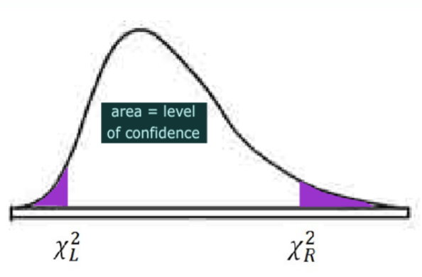
• Confidence is NOT symmetric since chi‐square distribution is not symmetric.
• Take square root of both endpoints to get confidence interval for the population standard deviation (\(\sigma\)).  

\[\left(\dfrac{(n-1) s^{2}}{\chi_{R}^{2}}, \dfrac{(n-1) s^{2}}{\chi_{L}^{2}}\right) \nonumber \]

Example: Performance risk in finance

In performance measurement of investments, standard deviation is a measure of volatility or risk. Twenty monthly returns from a mutual fund show an average monthly return of 1 percent and a sample standard deviation of 5 percent. Find a 95% confidence interval for the monthly standard deviation of the mutual fund.

Solution

The Chi‐square distribution will have 20‐1 =19 degrees of freedom. Using technology, we find that the two critical values are \(\chi_{L}^{2}=8.90655\) and  \(\chi_{R}^{2}=32.8523\)

Formula for confidence interval for \(\sigma\) is: \(\left(\sqrt{\dfrac{(19) 5^{2}}{32.8523}}, \sqrt{\dfrac{(19) 5^{2}}{8.90655}}\right)=(3.8,7.3)\)

One can say with 95% confidence that the standard deviation for this mutual fund is between 3.8 and 7.3 percent per month.