21.2: Estimating Posterior Distributions (Section 20.4)
- Page ID
- 8830

\( \newcommand{\vecs}[1]{\overset { \scriptstyle \rightharpoonup} {\mathbf{#1}} } \) \( \newcommand{\vecd}[1]{\overset{-\!-\!\rightharpoonup}{\vphantom{a}\smash {#1}}} \)\(\newcommand{\id}{\mathrm{id}}\) \( \newcommand{\Span}{\mathrm{span}}\) \( \newcommand{\kernel}{\mathrm{null}\,}\) \( \newcommand{\range}{\mathrm{range}\,}\) \( \newcommand{\RealPart}{\mathrm{Re}}\) \( \newcommand{\ImaginaryPart}{\mathrm{Im}}\) \( \newcommand{\Argument}{\mathrm{Arg}}\) \( \newcommand{\norm}[1]{\| #1 \|}\) \( \newcommand{\inner}[2]{\langle #1, #2 \rangle}\) \( \newcommand{\Span}{\mathrm{span}}\) \(\newcommand{\id}{\mathrm{id}}\) \( \newcommand{\Span}{\mathrm{span}}\) \( \newcommand{\kernel}{\mathrm{null}\,}\) \( \newcommand{\range}{\mathrm{range}\,}\) \( \newcommand{\RealPart}{\mathrm{Re}}\) \( \newcommand{\ImaginaryPart}{\mathrm{Im}}\) \( \newcommand{\Argument}{\mathrm{Arg}}\) \( \newcommand{\norm}[1]{\| #1 \|}\) \( \newcommand{\inner}[2]{\langle #1, #2 \rangle}\) \( \newcommand{\Span}{\mathrm{span}}\)\(\newcommand{\AA}{\unicode[.8,0]{x212B}}\)
# create a table with results
nResponders <- 64
nTested <- 100

drugDf <- tibble(
  outcome = c("improved", "not improved"),
  number = c(nResponders, nTested - nResponders)
)
Computing likelihood
likeDf <-
  tibble(resp = seq(1,99,1)) %>%
  mutate(
    presp=resp/100,
    likelihood5 = dbinom(resp,100,.5),
    likelihood7 = dbinom(resp,100,.7),
    likelihood3 = dbinom(resp,100,.3)
)

ggplot(likeDf,aes(resp,likelihood5)) +
  geom_line() +
  xlab('number of responders') + ylab('likelihood') +
  geom_vline(xintercept = drugDf$number[1],color='blue') +
  geom_line(aes(resp,likelihood7),linetype='dotted') +
  geom_line(aes(resp,likelihood3),linetype='dashed')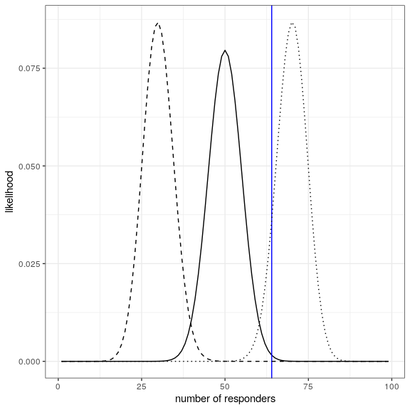
Computing marginal likelihood
# compute marginal likelihood
likeDf <-
  likeDf %>%
  mutate(uniform_prior = array(1 / n()))

# multiply each likelihood by prior and add them up
marginal_likelihood <-
  sum(
    dbinom(
      x = nResponders, # the number who responded to the drug
      size = 100, # the number tested
      likeDf$presp # the likelihood of each response
    ) * likeDf$uniform_prior
  )
Comuting posterior
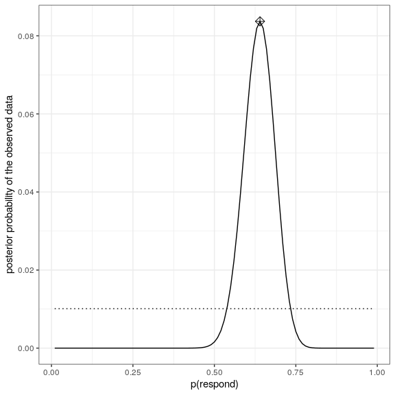
bayesDf <-
  tibble(
    steps = seq(from = 0.01, to = 0.99, by = 0.01)
  ) %>%
  mutate(
    likelihoods = dbinom(
      x = nResponders,
      size = 100,
      prob = steps
    ),
    priors = dunif(steps) / length(steps),
    posteriors = (likelihoods * priors) / marginal_likelihood
  )

# compute MAP estimate
MAP_estimate <-
  bayesDf %>%
  arrange(desc(posteriors)) %>%
  slice(1) %>%
  pull(steps)


ggplot(bayesDf,aes(steps,posteriors)) +
  geom_line() +
  geom_line(aes(steps,priors),
            color='black',
            linetype='dotted') +
  xlab('p(respond)') +
  ylab('posterior probability of the observed data') +
  annotate(
    "point",
    x = MAP_estimate,
    y = max(bayesDf$posteriors),
    shape=9,
    size = 3
  )