Diagnostics for residuals(continued)

Last updated
Save as PDF

Page ID: 230

$ \newcommand{\vecs}[1]{\overset { \scriptstyle \rightharpoonup} {\mathbf{#1}} } $

$ \newcommand{\vecd}[1]{\overset{-\!-\!\rightharpoonup}{\vphantom{a}\smash {#1}}} $

$ \newcommand{\id}{\mathrm{id}}$ $ \newcommand{\Span}{\mathrm{span}}$

( \newcommand{\kernel}{\mathrm{null}\,}\) $ \newcommand{\range}{\mathrm{range}\,}$

$ \newcommand{\RealPart}{\mathrm{Re}}$ $ \newcommand{\ImaginaryPart}{\mathrm{Im}}$

$ \newcommand{\Argument}{\mathrm{Arg}}$ $ \newcommand{\norm}[1]{\| #1 \|}$

$ \newcommand{\inner}[2]{\langle #1, #2 \rangle}$

$ \newcommand{\Span}{\mathrm{span}}$

$ \newcommand{\id}{\mathrm{id}}$

$ \newcommand{\Span}{\mathrm{span}}$

$ \newcommand{\kernel}{\mathrm{null}\,}$

$ \newcommand{\range}{\mathrm{range}\,}$

$ \newcommand{\RealPart}{\mathrm{Re}}$

$ \newcommand{\ImaginaryPart}{\mathrm{Im}}$

$ \newcommand{\Argument}{\mathrm{Arg}}$

$ \newcommand{\norm}[1]{\| #1 \|}$

$ \newcommand{\inner}[2]{\langle #1, #2 \rangle}$

$ \newcommand{\Span}{\mathrm{span}}$ $ \newcommand{\AA}{\unicode[.8,0]{x212B}}$

$ \newcommand{\vectorA}[1]{\vec{#1}} % arrow$

$ \newcommand{\vectorAt}[1]{\vec{\text{#1}}} % arrow$

$ \newcommand{\vectorB}[1]{\overset { \scriptstyle \rightharpoonup} {\mathbf{#1}} } $

$ \newcommand{\vectorC}[1]{\textbf{#1}} $

$ \newcommand{\vectorD}[1]{\overrightarrow{#1}} $

$ \newcommand{\vectorDt}[1]{\overrightarrow{\text{#1}}} $

$ \newcommand{\vectE}[1]{\overset{-\!-\!\rightharpoonup}{\vphantom{a}\smash{\mathbf {#1}}}} $

$ \newcommand{\vecs}[1]{\overset { \scriptstyle \rightharpoonup} {\mathbf{#1}} } $

$ \newcommand{\vecd}[1]{\overset{-\!-\!\rightharpoonup}{\vphantom{a}\smash {#1}}} $

$\newcommand{\avec}{\mathbf a}$ $\newcommand{\bvec}{\mathbf b}$ $\newcommand{\cvec}{\mathbf c}$ $\newcommand{\dvec}{\mathbf d}$ $\newcommand{\dtil}{\widetilde{\mathbf d}}$ $\newcommand{\evec}{\mathbf e}$ $\newcommand{\fvec}{\mathbf f}$ $\newcommand{\nvec}{\mathbf n}$ $\newcommand{\pvec}{\mathbf p}$ $\newcommand{\qvec}{\mathbf q}$ $\newcommand{\svec}{\mathbf s}$ $\newcommand{\tvec}{\mathbf t}$ $\newcommand{\uvec}{\mathbf u}$ $\newcommand{\vvec}{\mathbf v}$ $\newcommand{\wvec}{\mathbf w}$ $\newcommand{\xvec}{\mathbf x}$ $\newcommand{\yvec}{\mathbf y}$ $\newcommand{\zvec}{\mathbf z}$ $\newcommand{\rvec}{\mathbf r}$ $\newcommand{\mvec}{\mathbf m}$ $\newcommand{\zerovec}{\mathbf 0}$ $\newcommand{\onevec}{\mathbf 1}$ $\newcommand{\real}{\mathbb R}$ $\newcommand{\twovec}[2]{\left[\begin{array}{r}#1 \\ #2 \end{array}\right]}$ $\newcommand{\ctwovec}[2]{\left[\begin{array}{c}#1 \\ #2 \end{array}\right]}$ $\newcommand{\threevec}[3]{\left[\begin{array}{r}#1 \\ #2 \\ #3 \end{array}\right]}$ $\newcommand{\cthreevec}[3]{\left[\begin{array}{c}#1 \\ #2 \\ #3 \end{array}\right]}$ $\newcommand{\fourvec}[4]{\left[\begin{array}{r}#1 \\ #2 \\ #3 \\ #4 \end{array}\right]}$ $\newcommand{\cfourvec}[4]{\left[\begin{array}{c}#1 \\ #2 \\ #3 \\ #4 \end{array}\right]}$ $\newcommand{\fivevec}[5]{\left[\begin{array}{r}#1 \\ #2 \\ #3 \\ #4 \\ #5 \\ \end{array}\right]}$ $\newcommand{\cfivevec}[5]{\left[\begin{array}{c}#1 \\ #2 \\ #3 \\ #4 \\ #5 \\ \end{array}\right]}$ $\newcommand{\mattwo}[4]{\left[\begin{array}{rr}#1 \amp #2 \\ #3 \amp #4 \\ \end{array}\right]}$ $\newcommand{\laspan}[1]{\text{Span}\{#1\}}$ $\newcommand{\bcal}{\cal B}$ $\newcommand{\ccal}{\cal C}$ $\newcommand{\scal}{\cal S}$ $\newcommand{\wcal}{\cal W}$ $\newcommand{\ecal}{\cal E}$ $\newcommand{\coords}[2]{\left\{#1\right\}_{#2}}$ $\newcommand{\gray}[1]{\color{gray}{#1}}$ $\newcommand{\lgray}[1]{\color{lightgray}{#1}}$ $\newcommand{\rank}{\operatorname{rank}}$ $\newcommand{\row}{\text{Row}}$ $\newcommand{\col}{\text{Col}}$ $\renewcommand{\row}{\text{Row}}$ $\newcommand{\nul}{\text{Nul}}$ $\newcommand{\var}{\text{Var}}$ $\newcommand{\corr}{\text{corr}}$ $\newcommand{\len}[1]{\left|#1\right|}$ $\newcommand{\bbar}{\overline{\bvec}}$ $\newcommand{\bhat}{\widehat{\bvec}}$ $\newcommand{\bperp}{\bvec^\perp}$ $\newcommand{\xhat}{\widehat{\xvec}}$ $\newcommand{\vhat}{\widehat{\vvec}}$ $\newcommand{\uhat}{\widehat{\uvec}}$ $\newcommand{\what}{\widehat{\wvec}}$ $\newcommand{\Sighat}{\widehat{\Sigma}}$ $\newcommand{\lt}{<}$ $\newcommand{\gt}{>}$ $\newcommand{\amp}{&}$ $\definecolor{fillinmathshade}{gray}{0.9}$

Diagnostics for residuals (continued)

Nonnormality of errors

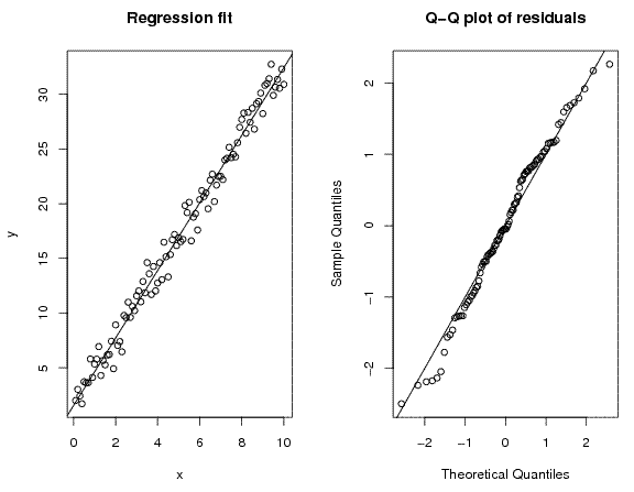
This can be studied graphically by using the normal probability plot, or Q-Q (standing for quantile-quantile) plot. In this plot, the ordered residual (or observed quantiles) of the residuals are plotted aginst the expected quantiles assuming that $\epsilon_i$'s are approximately normal and independent with mean 0 and variance = MSE. This results in plotting the k-th largest e_i against

$${\sqrt{MSE}*z\left[\dfrac{k-0.375}{n+0.25}\right]},$$

where z(q) is the q-th quantile of N(0,1) distribution, where0<q<1. If the errors are normally distributed then the points on the plots should almost along the diagonal line. Departures from that could indicates skewness or heavier-tailed distributions.

(a) The model: $Y = 2 + 3X + \epsilon$, where $\epsilon$~N(0,1). 100 observations, with Xi= i/10, i = 1,...,100

Coefficients	Estimate	Std. Error	t-statistic	P-value
Intercept	1.5413	0.2196	7.02	2.92 * 10^-10
Slope	3.08907	0.03775	81.84	<2 * 10^-16

$${\sqrt{MSE}}$$= 1.09, R2 = 0.9856.

(b) True Model: $ Y = 2+3X+\epsilon$, where $\epsilon$~t5.. 100 observations, with Xi = i/10, i = 1...100.

Coefficients	Estimate	Std. Error	t-statistic	P-value
Intercept	2.11144	0.28279	7.467	3.42*10^-11
Slope	2.97458	0.04862	61.185	<2*10^-16

$${\sqrt{MSE}} = 1.403,$$

with $R^2 = 1.403$.

Coefficients	Estimate	Std. Error	t-statistic	P-value
Intercept	2.4615	0.6533	3.768	0.000281
Slope	2.9894	0.1123	26.617	<2*10^-16

$${\sqrt{MSE}}$$ = 3.242, R2 = 0.8785.

(d) True Model:$Y = 2+3X+\epsilon$. where $\epsilon$ ~ (5-x52). 100 observations, with Xi = i/10, i= 1...100.

Coefficients	Estimate	Std. Error	t-statistic	P-value
Intercept	2.7402	0.4694	6.838	6.87*10^-8
Slope	2.9896	0.0807	37.048	<2*10^-16

$${\sqrt{MSE}}= 2.329,$$

with $R^2 = 0.9334$.

Heteroscedasticity

Heteroscedasticity or unequal variance: the variance of the error $\epsilon$i may sometimes depend on the value of Xi. This is often reflected in the plot of residuals versus X through an unequal spread of the residuals along the X-axis.

One possibility is that the variance either increases or decreases with increasing value of X. This is often true for financial data, where the volume of transactions usually has a role in the uncertainty of the market. Another possibility is that the data may come from different strata with different variabilities. E.g. different measuring instruments, with different precisions, may have been used.

(a) True Model:$Y = 2+3X+\epsilon$. where $\epsilon$ ~ (5-x52). 100 observations, with Xi = i/10, i= 1...100.

Coefficients	Estimate	Std. Error	t-statistic	P-value
Intercept	1.0074	0.9729	1.035	0.303
Slope	3.3382	0.1673	19.958	<2*10^-16

$${\sqrt{MSE}}$$ = 2.329, R2 = 0.9334.

Contributors

Chengcheng Zhang

Search

Text Color

Text Size

Margin Size

Font Type