Nonparametric Inference - Kernel Density Estimation

Introduction and definition

Here we discuss the non-parametric estimation of a pdf \(f\) of a distribution on the real line. The kernel density estimator is a non-parametric estimator because it is not based on a parametric model of the form \( \{ f_{\theta}, \theta \in \Theta \subset {\mathbb R}^d\} \). What makes the latter model 'parametric' is the assumption that the parameter space \(\Theta\) is a subset of \({\mathbb R}^d\) which, in mathematical terms, is a finite-dimensional space. In such a parametric case, all we need to do is to estimate finitely many (i.e. d) parameters and this then specifies our density estimator entirely. A typical example for such a parametric model is the normal model, where \(\theta = (\mu,\sigma^2).\) In such a model we only need to estimate the two parameters (via least squares, for instance), and then we know how the density looks like based on these estimated parameters (see also the discussion of effective sample size below).

A non-parametric approach is used if very little information about the underlying distribution is available, so that the specification of a parametric model cannot be well justified. Non-parametric models are much broader than parametric models. The model underlying a kernel density estimator usually only assumes that the data are sampled from a distribution that has a density f satisfying some 'smoothness' conditions, such as continuity, or differentiability. [One should mention here that in general the line between parametric and non-parametric procedures is not as clear as it might sound. A kernel density estimator is clearly a non-parametric estimator, however.]

A kernel density estimator based on a set of n observations \(X_1,\ldots,X_n\) is of the following form:

\[ {\hat f}_n(x) = \frac{1}{nh} \sum_{i=1}^n K\Big(\frac{X_i - x}{h}\Big) \]

where h > 0 is the so-called {\em bandwidth}, and K is the kernel function, which means that \(K(z) \ge 0\) and \(\int_{\mathbb R} K(z) dz = 1,\) and usually one also assumes that K is symmetric about 0. The choice of both the kernel and the bandwidth is left to the user. The choice of the latter is quite crucial (see also discussion of optimal bandwidth choice below), whereas the choice of the kernel tends to have a relatively minor effect on the estimator. In order to understand why the just given formula describes a reasonable estimator for a pdf let us consider a simple example.

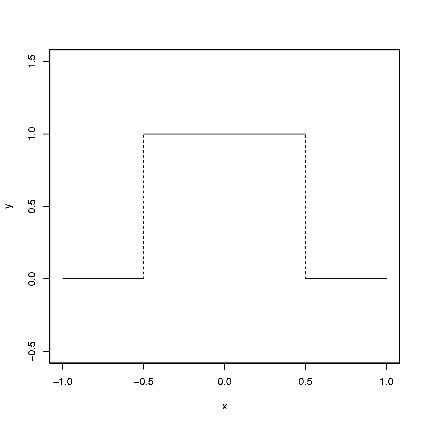
The kernel density estimator using a rectangular kernel

A 'rectangular kernel' K is given by the pdf of a uniform distribution on the interval \( (-\frac{1}{2}, \frac{1}{2})\), which is of the form

$$ K(z) = \begin{cases}1 & \text{for }\; -{\textstyle \frac{1}{2} < z < \frac{1}{2}}\\0 & \text{otherwise.}\end{cases} $$

How does our kernel density estimator look like with this choice of K? To see this, first observe that for the rectangular kernel we have that \( K\big(\frac{X_i - x}{h}\big) \) is either 1 or 0 depending on whether \( -\frac{1}{2} < \frac{X_i - x}{h} < \frac{1}{2} \) holds or not. Using simple algebra one can see that this condition holds if and only if

$$ x - \frac{h}{2} < X_i < x + \frac{h}{2}.$$

This in turn means that the sum \(\sum_{i=1}^n K\big(\frac{X_i - x}{h}\big)\) equals the number of observations X_i that fall into the interval (x-h/2, x + h/2), because we are summing only 1's and 0's, and consequently the sum equals the number of 1's, which is the same as the number of observations falling into \( (x-\frac{h}{2},x+\frac{h}{2} ) \).

We now see that the kernel density estimator with a rectangular kernel is of the form

$$\widehat{f}_n(x) = \frac{\text{average number of observations in }\,(x-\frac{h}{2},x+\frac{h}{2})}{h}.$$

Noticing that h is the length of the interval \( (x-\frac{h}{2},x+\frac{h}{2} ) \) then this equals the average number of observations in the `bin' \( (x-\frac{h}{2},x+\frac{h}{2} ) \) divided by the length of the bin. Of course the well-known histogram is exactly of this form. However, for a histogram we have only a finite, fixed number of prespecified bins, whereas here in case of a kernel density estimator using a rectangular kernel the bin itself depends on x. In particular, in contrast to a histogram, close by bins are overlapping.

Another important remark is here in order. The kernel density estimate at x only depends on the observations that fall close to x (inside the bin \( (x-\frac{h}{2},x+\frac{h}{2}) \) ).This makes sense because the pdf is a derivative of the cdf and the derivative of F at x only depends on the behavior of F locally at the point x and this local bevahior of F at x is reflected by the number of points falling into a small bin centered at x. Now, it is clear that not all the n available observations fall into a small bin around a given point x, and so the quality of the kernel density estimator (in terms of variance) at a given point x cannot be expected to be as good as in the case of the estimator of a (global) parameter that uses all the available observations. (See discussion on 'effective sample size' given below.)

The step from a rectangular kernel to a general kernel is now motivated by the fact that since the rectangular kernel is not continuous (it has two jumps at \( -\frac{1}{2} \) and \( \frac{1}{2} \), respectively), the resulting kernel estimator is also not continuous. Therefore one often uses a continuous kernel function. Since sums of continuous (or differentiable) functions are again continuous (or differentiable), the resulting kernel density estimator then is continuous. Another way to think about a more general kernel is to observe that the rectangular kernel gives a weight of either 1 or 0 to each observation (depending on whether \(X_i\) falls into \( (x-\frac{h}{2},x+\frac{h}{2}) \) or not). It might be a better idea to replace these simple 0-1-weights by more general weights that decrease smoothly when moving away from x in either direction. Such kernels K might have a compact support (for instance, K(z) > 0 only on an interval (a,b) with a < b, and K(z) = 0 otherwise) or not. They might even have a strictly positive value everywhere, such as the standard normal pdf, which in fact is a popular kernel function.

Kernel density estimation with R

(To be added.)

The bias and the variance of a kernel density estimator

Notice that \(\hat{f}_n(x)\) in fact is a function (in x), but when we speak of bias and variance of the kernel estimator then we mean the random quantity \(\hat{f}_n(x)\) for a fixed value of x.

In order to be able to do bias and variance calculations we obviously need to specify the sampling distribution. Here we consider the standard case that the observations \(X_1,\ldots,X_n\) constitute a random sample, i.e. they are independent and have identical distribution (iid) given by the pdf f. First we again consider the special case of a rectangular kernel, because in this case finding nice expressions bias and variance does not require calculus but only some based knowledge of probability.

We have seen that for a rectangular kernel we have

$$n\,h\, \hat{f}_n(x) = \text{number of observations in }\,{\textstyle (x-\frac{h}{2},x+\frac{h}{2})}.$$

(Notice that as compared to the above we multiplied both sides by \( n\,h. \)) Since the observations are assumed to be iid, we see that the right hand side (and thus also the left hand side) is in fact a random variable that has a binomial distribution, because it is the number of successes in a sequence of n Bernoulli trials where each trial has only one of two outcomes 1 or 0 (success or failure). Success of the i-th trial here means that \(X_i\) falls into the bin \( (x-\frac{h}{2},x+\frac{h}{2})\). The success probability p of the Bernoulli trials thus is given by the probability content of the interval \( (x-\frac{h}{2},x+\frac{h}{2})\) under the pdf f, which, in other words, is the integral of f over this interval. In terms of the cdf F we can express this as \( p = F(x-\frac{h}{2}) - F(x-\frac{h}{2}) \).

We have thus arrived at the conclusion that

$$n\,h\,\hat{f}_n(x) \sim \text{Bin}{\textstyle \big(n, F(x+\frac{h}{2}\,) - F(x-\frac{h}{2}\,)\,\big)},$$

where the notation \(Z \sim \text{Bin}(n,p) \) means that the distribution of the random variable Z is a binomial with parameters n and p.
It is well-known that a binomial distribution with parameters n and p has mean np. We therefore obtain that \( \text{E}(nh\ \hat{f}_n(x)) = n\, \big( F(x+{\textstyle\frac{h}{2}}\,) - F(x-{\textstyle\frac{h}{2}}\,) \big)\), or, by dividing by nh,

\[ \text{E}\big(\hat{f}_n(x)\big) = \frac{F(x+{\textstyle\frac{h}{2}}\,) - F(x-{\textstyle\frac{h}{2}}\,)}{h} \]

Let's pause a little, and discuss this. What we want to estimate by using \(\hat{f}_n(x)\) is \(f(x)\), the value of the underlying pdf at x. Our calculations show that the expected value E\(\big(\hat{f}_n(x)\big) \) in general does not equal f(x). In statistical terms this means that the kernel density estimator is biased:

\[ \text{bias} \big( \hat{f}_n(x) \big) = \text{E}( \hat{f}_n(x) ) - f(x) \ne 0. \]

However, if the cdf F is differentiable at x, then by definition of differentiability we have that

\[ \frac{F(x+{\textstyle\frac{h}{2}}\,) - F(x-{\textstyle\frac{h}{2}}\,)}{h} \to f(x) \quad \text{ as } h \to 0 \]

and thus the bias will tend to be close to 0 if h is small.

It is important to observe here that in practice for a given sample size the bandwidth h cannot be chosen too small, because otherwise none of the observations will fall into the bin \(x-\frac{h}{2}\) and \(x+\frac{h}{2}\), leading to a useless estimator of the pdf. On the other hand if the sample size is large, and h is not 'sufficiently' small, then the estimator will stay biased as we have indicated above. The `right' choice of the bandwidth is a challenge, but it is hopefully clear from this discussion that the choice of h also needs to depend on the sample size n. Mathematically, we think of \(h = h_n\) being a sequence satisfying

\[ h_n \to 0 \quad \text{ as } n \to \infty. \]

Now let's discuss the variance of the kernel density estimator (still based on the rectangular kernel). Using again the fact that \( n\,h\,\hat{f}_n(x)\) is a Bin(n,p) random variable, and recalling the fact that the variance of a Bin(n,p) distribution equals np(1-p) we have by using the shorthand notation \( F(\,x-\frac{h}{2},\,x+\frac{h}{2}\,) = F(x+\frac{h}{2}\,) - F(x-\frac{h}{2}) \) that

\[ {\textstyle\text{Var}(nh \hat f_n(x)) = n\,\, F\big(\, x- \frac{h}{2},\,x+\frac{h_n}{2}\,\big)\,\big(\,1 - F\big(\,x-\frac{h}{2},\,x+\frac{h}{2}\,\big)\,\big) }\]

and by using the fact that Var\((cZ) = c^2\text{Var}(Z)\) for a constant c we obtain

\[ {\textstyle \text{Var}(\hat f_n(x)) = \big( \frac{1}{nh} \big)^2 n\,\, F\big(\, x- \frac{h}{2},\,x+\frac{h}{2}\,\big)\,\big(\,1 - F\big(\,x-\frac{h}{2},\,x+\frac{h}{2}\,\big)\,\big) }\]

In order to make more sense out of this, we rewrite this formula as:

\[ \text{Var}(\hat f_n(x)) = \frac{1}{nh} \, \frac{ F\big(\, x- {\textstyle \frac{h}{2},\,x+\frac{h}{2}}\,\big)}{h}\,\big(\,1 - F\big( x-{\textstyle \frac{h}{2},\,x+\frac{h}{2}}\,\big)\,\big) \tag{*} \]

Now observe that for small values of h (and this is what we need for the bias to be small as well), the last term \( 1 - F\big( x-{\textstyle \frac{h}{2},\,x+\frac{h}{2}}\,\big)\) is close to 1 (because the expression \(F\big( x-{\textstyle \frac{h}{2},\,x+\frac{h}{2}}\,\big)\) equals the probability that an observation falls into the interval \( \big( x-{\textstyle \frac{h}{2},\,x+\frac{h}{2}}\,\big)\), which by definition of a pdf equals the area under the pdf f between \(x-\frac{h}{2}\) and \(x+\frac{h}{2}\), and for small h these two bounds are very close together, so that the area under the curve also is small. Of course, this is loosely formulated. From a mathematical point of view we mean that

\[ 1 - F\big( x-{\textstyle \frac{h}{2},\,x+\frac{h}{2}}\,\big) \to 1\quad \text{ as } h \to 0. \]

What about the second term in (*)? Again using the interpretation of \( F\big(\, x- {\textstyle \frac{h}{2},\,x+\frac{h}{2}}\,\big)\) as the area under the curve f between the bounds \(x-\frac{h}{2}\) and \(x+\frac{h}{2}\), we see that if the interval given by these two bounds is small, then this area is approximately equal to the area of the rectangle with height f(x) and width being the length of the interval, which is h, so that \( F\big(\, x- {\textstyle \frac{h}{2},\,x+\frac{h}{2}}\,\big) \approx f(x) h\). In other words, the second term in (*) satisfies

\[ \frac{ F\big(\, x- {\textstyle \frac{h}{2},\,x+\frac{h}{2}}\,\big)}{h} \to f(x)\quad \text{ as } h \to 0. \]

Assuming that x is such that f(x) > 0 (strictly), we conclude that for small values of h the variance of the kernel estimator evaluated at x behaves like

\[ \text{Var}(\hat{f}_n(x)) \approx \frac{1}{nh} f(x). \tag{**}\]

Now, if we want our kernel density estimator \(\hat{f}_n(x)\) to be a consistent estimator for f(x), meaning that \(\hat{f}_n(x)\) is `close' to f(x) at least if the sample size n is large (more precisely, \(\hat{f}_n(x)\) converges to f(x) in probability as \(n \to \infty\)), then we want to have both, the bias tending to zero and the variance tending to zero as the sample size tends to infinity. We have seen above that for the former we need that

\[h = h_n \to 0 \quad \text{ as } n \to \infty \quad \text{ in order for the bias to become small for large sample size}\]

and from (**) we can see that for the latter we need that \(h = h_n\) is such that

\[ nh_n \to \infty\quad\text{ as } n \to \infty \quad \text{ in order for the variance to become small for large sample size}\]

These two conditions on the bandwidth are standard when the behavior of the kernel estimator is analyzed theoretically. Similar formulas can be derived for more general kernel functions, but some more calculus is needed for that. (To be added.)

The bias-variance trade-off and 'optimal' bandwidth choice

The bias-variance trade-off is the uncertainty principle of statistics, and it shows up in many contexts. In order to understand this it is helpful to consider the decomposition of the mean squared error of an estimator into squared bias and variance. Since we are dealing with kernel estimation here, we use the estimator \(\hat{f}_n(x)\), but the decomposition holds for any estimator (with finite variance). The mean squared error of \(\hat{f}_n(x)\) is defined as

\[ \text{MSE}(\hat{f}_n(x)) = \text{E}\big( \hat{f}_n(x) - f(x)\big)^2. \]

The mean squared error is a widely accepted measure of quality of an estimator. The following decomposition holds:

\[ \text{MSE}(\hat{f}_n(x)) = \text{Var}(\hat{f}_n(x)) + \big[\text{bias}\big(\hat{f}_n(x)\big)\big]^2. \]

The proof of this decomposition is given below. Note that this in particular tells us that if our estimator is unbiased (bias = 0), then the MSE reduces to the variance. (Classical estimation theory deals with unbiased estimators and thus the variance is used there as a measure of performance.)

Now observe that the above calculations of bias and variance indicate (at least intuitively) that

• the bias of \(\hat{f}_n(x)\) increases as h increases, since we are estimating \(\frac{F\big(x+\frac{h}{2}\big) - F\big(x-\frac{h}{2}\big)}{h}\), and
• the variance of \(\hat{f}_n(x)\) increases as h decreases, since fewer observations are included into the estimation process, and averaging over fewer (independent) observations decreases the variance.

The last statement is based on the following fact. If \(X_1,\ldots,X_n\) is a random sample with \(\text{Var}(X_1) = \sigma^2 < \infty\) then the variance of the average of the \(X_i\)'s, i.e. the variance of \(\overline{X}_n = \frac{1}{n}\sum_{i=1}^n X_i\) equals

\[{\text Var}(\overline{X}_n) = \text{Var}\big(\frac{1}{n} \sum_{i=1}^n X_i\big) = \frac{1}{n^2}\text{Var}\big(\sum_{i=1}^n X_i\big) = \frac{1}{n^2} n \sigma^2 = \frac{1}{n} \sigma^2.\]

So the variance is de(in)creasing when we in(de)crease the number of (independent) variables we averge.

Oversmoothing and undersmoothing

Now, considering the above two bullet points we see that in order to minimize the MSE of \(\hat{f}_n(x)\) we have to strike a balance between bias and variance by an appropriate choice of the bandwidth h (`not too small and not too big'). If h is large, then the bias is large, because we are in fact `averaging' over a large neighborhood of x, and as discussed above, the expected value of the kernel estimator is the area under the curve (i.e. under f) over the bin \(x- \frac{h}{2}, x + \frac{h}{2}\) divided by the length of this bin, namely h. This means the larger the bin is, the further away from f(x) we can expect the mean to be. Choosing a bandwidth that is too large is called oversmoothing and this means a large bias. The other extreme is choosing a bandwidth that is too small (undersmoothing). In this case the bias is small, but the variance is large. Striking the right balance is an art.

Optimal bandwidth choice

Using some more assumptions on f we can get a more explicit expression for how the bias depends on h. In the case of a rectangular kernel we have seen that \( \text{bias}\big(\hat{f}_n(x)\big) = \frac{F\big(x+\frac{h}{2}\big) - F\big(x-\frac{h}{2}\big)}{h} - f(x)\). We can write the numerator in this expression as \(\big[F\big(x+\frac{h}{2}\big) - F(x)\big] - \big[F\big(x-\frac{h}{2}\big) - F(x)\big]\). If we assume that f is twice differentiable then we can use a two-term Taylor expansion to both of the differences in the brackets to get

\[ F\big(x+{\textstyle \frac{h}{2}}\big) - F(x) = f(x) {\textstyle \frac{h}{2}} + {\textstyle \frac{1}{2}}\, f^\prime(x) \big({\textstyle \frac{h}{2}}\big)^2 + {\textstyle\frac{1}{3!}}\,f^{\prime\prime}(x) \big({\textstyle \frac{h}{2}}\big)^3 \]

and similarly

\[ F\big(x-{\textstyle \frac{h}{2}}\big) - F(x) = f(x) \big(- {\textstyle \frac{h}{2}}\,\big)+ {\textstyle \frac{1}{2}}\, f^\prime(x) \big(-{\textstyle \frac{h}{2}}\big)^2 + {\textstyle\frac{1}{3!}}\,f^{\prime\prime}(x) \big(-{\textstyle \frac{h}{2}}\big)^3 \].

Taking their difference gives

\[F\big(x+\frac{h}{2}\big) - F\big(x-\frac{h}{2}\big) = f(x) h + {\textstyle \frac{1}{6}}\, f^{\prime\prime}(x) h^3 \]

so that the bias satisfies

\[ \text{bias}(\hat{f}_n(x)) = \frac{F\big(x+\frac{h}{2}\big) - F\big(x-\frac{h}{2}\big)}{h} - f(x) \approx {\textstyle \frac{1}{24}}\, f^{\prime\prime}(x) h^2,\]

where we used '\(\approx\)' rather than '\(=\)' because we ignored the remainder terms in the Taylor expansion. Even if we are using more general kernels, as long as we assume them to be symmetric about 0, and as long as f is twice differentiable at x, one can show a similar epansion of the bias, namely, that the bias approximately equals a constant times \(f^{\prime\prime}(x) h^2\). This, together with the above approximation of the variance can then be used to balance out (squared) bias and variance in order to find the bandwidth minimizing the MSE as follows. We have the approximation

\[\text{MSE}(\hat{f}_n(x)) = \text{Var}(\hat{f}_n(x)) + \text{bias}^2(\hat{f}_n(x)) \approx c_1 {\textstyle \frac{1}{nh}}\, f(x) + c_2 \big(f^{\prime\prime}(x)\big)^2 h^4.\]

where these constants depend on the kernel. in the case of a rectangular kernel we have seen that \(c_1 = 1\) and \(c_2 = \big(\frac{1}{24}\big)^2\). More generally, for other symmetric kernels these constants can be show to be \(c_1 = \frac{1}{4}\big(\int x^2K(x)dx\big)^2 \) and \(c_2 = \int K^2(x)dx\). We can easily minimize the right-hand side with respect to h by taking derivatives to get the bandwidth \(h_{loc}^*\) minimizing this right-hand side as

\[ h_{loc}^* = c_{loc}^* n^{-1/5},\]

where \(c_{loc}^* = \big( \frac{c_1}{4 c_2} \frac {f(x)} { (f^{\prime\prime}(x))^2 } \big)^{1/5}.\) This is known as the locally (asymptotically) optimal bandwidth of the kernel density estimator assuming that f is twice differentiable. It is locally optimal because it depends on the value x, and it is asymptotic because our approximations required a small value of h (recall that we ignored the remainder terms in the Taylor expansions), and since \(h = h_n \to 0\) as \(n \to \infty\) (see above) this means that implicitly we assume a large enough sample size n.

To use a different bandwidth for every different value of x is computationally not feasible (sometimes it does make sense, however, to use different bandwidths in different regions of f if these regions are expected to differ in their smoothness properties). Replacing the MSE by the integrated MSE (integrated over all values of x, there the integration is often done with respect to a weight function) gives a global measure for the performance of our kernel density estimator, and it turns out that similar calculations can be used to derive a globally optimal bandwidth which has the same form as the locally optimal bandwidth, namely

\[h^*_{glob} = c_{glob}^* n^{-1/5},\]

where the values of \(f(x)\) and \(f^{\prime\prime}(x)\) in \(c^*_{loc}\) are replaced by integrated versions. We still cannot use this in practice, because the constant \(c_{glob}^*\) depends on the unknown quantities, namely the (weighted) integrals of \(f(x)\) and \(f^{\prime\prime}(x)\), respectively. There are various practical ways of how to obtain reasonable values for \(c^*_{glob}\). One of them is to estimate the constant \(c_{glob}^*\), for instance by estimating \(f(x)\) and \(f^{\prime\prime}(x)\) via kernel estimators. Another often used approach is to use a reference distribution in determining \(c^*_{glob}\), such as the normal distribution. This means, one first estimates mean and variance from the data, and then uses the corresponding normal to find the corresponding values of the weighted integrals.

proof of the decomposition of the MSE:

Write \(\text{MSE}(\hat{f}_n(x)) = \text{E}(\hat{f}_n(x) - f(x))^2 = \text{E}\big([\hat{f}_n(x) - \text{E}(\hat{f}_n(x))] + [\text{E}(\hat{f}_n(x)) - f(x)]\big)^2\). Nothing really happened. We only added and subtracted the term \(\text{E}(\hat{f}_n(x))\) (and included some brackets). Now we expand the square (by keeping the terms in the brackets together) and use the fact that the expectation of sums equals the sum of the expectations, i.e. we use that \(\text{E}(X+Y) = \text{E}(X) + \text{E}(Y)\) (and of course this holds with any finite number of summands). This then gives us

\[ \text{MSE}(\hat{f}_n(x)) = \text{E}\big(\hat{f}_n(x) - \text{E}(\hat{f}_n(x)) \big)^2 + \text{E}\big( \text{E}(\hat{f}_n(x)) - f(x)]\big)^2 + \]

\[ 2 \text{E}\big( \big[\hat{f}_n(x) - \text{E}\big(\hat{f}_n(x)\big)\big] \cdot \big[\text{E}\big(\hat{f}_n(x)\big) - f(x) \big]\big).\]

The first term on the right-hand side equals Var\(\big(\hat{f}_n(x)\big)\). The second term is the expected value of a constant, which of course equals the constant itself, and this constant is the squared bias. So it remains to show that the third term on the right equals zero. Looking the the product inside the expectation of this term we see, that only one of the two terms is random, the other, namely \(\text{E}\big(\hat{f}_n(x)\big) - f(x)\) is a constant. To make this more clear, we replace this (long) constant term by the symbol c. So the third term becomes

\[ \text{E}\big( \big[\hat{f}_n(x) - \text{E}\big(\hat{f}_n(x)\big)\big] \cdot c \big) = c\,\text{E}\big( \hat{f}_n(x) - \text{E}\big(\hat{f}_n(x) \big) \]

and the last expectation is of the form \(\text{E}\big(Z - \text{E}(Z)\big)\) and again using the facts that the expectation of the sum equals the sums of the expectations we have \(\text{E}\big(Z - \text{E}(Z)\big) = \text{E}(Z) - \text{E}(Z) = 0.\) This completes the proof.

Effective sample size

From a statistical perspective an important distinction between a parametric and the non-parametric density estimator is the 'effective number of observations' that are used to estimate the pdf f at a specific point x. In the parametric case we use all the available data to estimate the parameters by \(\widehat{\theta}\), and the estimator of the pdf at the point x then simply is given by \( f_{\hat{\theta}}(x). \) This means that all the data are used to estimate f(x) at any given point x and thus the effective sample size for estimating f at a fixed point x equals the sample size n. Not so in the non-parametric case.

As we have discussed above, when using a rectangular kernel in the estimator \(\hat{f}_n(x)\), then we are only using those data that are falling inside a small neighborhood of the point x, namely inside the bin \(\big(x - \frac{h}{2} , x + \frac{h}{2}\big)\). How many points can we expect to fall into this bin? We have already done this calculation above based on the binomial distribution: The expected number of observations falling into the bin is np where

\[p = F\big(x + \frac{h}{2}\big) - F\big( x - \frac{h}{2}\big) .\]

Now, we also have seen already that

\[\frac{F\big(x + \frac{h}{2}\big) - F\big( x - \frac{h}{2}\big)}{h} \to f(x),\]

in other words,

\[ np = n\big(F\big(x + \frac{h}{2}\big) - F\big( x - \frac{h}{2}\big)\big) \approx f(x) n h.\]

Now both p and n depend on the sample size while f(x) is a constant. So ignoring this constant, the effective sample size is 'of the order' nh, which is also the order of the variance of the kernel estimator! This of course makes sense, because the kernel density estimator is in fact averaging over (in the mean) nh points (see the calculation of the variance of \(\overline{X}_n\)).

Since h is assumed to become small (tends to zero) as the sample size increases, the effective sample size for a kernel estimator is of smaller order than the sample size n, which is the effective sample size of parametric estimators of a density. This means that the performance of the kernel density estimator cannot be as good as the performance of a parametric estimator of a density (see also discussion at the beginning of this page). However, the kernel estimator 'works' under much weaker assumptions than the parametric estimator, and this is the basic trade-off between non-parametric and parametric methods, namely weak model assumptions and weak(er) performance of estimators on the one hand, versus strong model assumptions and strong performance of the estimator on the other. The derived performances of both of the estimators hold if the underlying model assumptions hold. Since the model assumptions in the parametric case are much stronger, we can be less certain that they actually hold (or that the assumptions constitute a 'good' approximation to the conditions under which the experiment is performed), but if they do, then the parametric estimator is not to beat by a nonparametric estimator.

Multivariate kernel density estimation and the curse of dimensionality

To be added.

Contributors

• Wolfgang Polonik